Page 94 - Basic Structured Grid Generation

Structured grid generation – algebraic methods 83

x = 1
x = 0

r
r 0 1
O

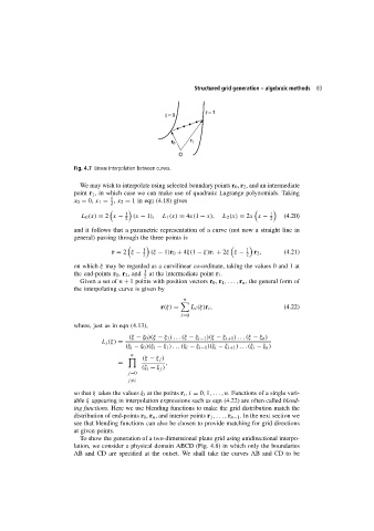
Fig. 4.7 Linear interpolation between curves.

We may wish to interpolate using selected boundary points r 0 , r 2 , and an intermediate
point r 1 , in which case we can make use of quadratic Lagrange polynomials. Taking
1
x 0 = 0, x 1 = , x 2 = 1 in eqn (4.18) gives
2

1 1
L 0 (x) = 2 x − (x − 1), L 1 (x) = 4x(1 − x), L 2 (x) = 2x x − (4.20)
2 2
and it follows that a parametric representation of a curve (not now a straight line in
general) passing through the three points is

1 1
r = 2 ξ − (ξ − 1)r 0 + 4ξ(1 − ξ)r 1 + 2ξ ξ − r 2 , (4.21)
2 2
on which ξ may be regarded as a curvilinear co-ordinate, taking the values 0 and 1 at
the end-points r 0 , r 2 ,and 1 at the intermediate point r 1 .
2
Given a set of n + 1 points with position vectors r 0 , r 1 ,... , r n , the general form of
the interpolating curve is given by
n

r(ξ) = L i (ξ)r i , (4.22)
i=0
where, just as in eqn (4.13),
(ξ − ξ 0 )(ξ − ξ 1 )...(ξ − ξ i−1 )(ξ − ξ i+1 )...(ξ − ξ n )
L i (ξ) =
(ξ i − ξ 0 )(ξ i − ξ 1 )... (ξ i − ξ i−1 )(ξ i − ξ i+1 ). ..(ξ i − ξ n )
n
(ξ − ξ j )

= ,
(ξ i − ξ j )
j=0
j =i
so that ξ takes the values ξ i at the points r i , i = 0, 1,..., n. Functions of a single vari-
able ξ appearing in interpolation expressions such as eqn (4.22) are often called blend-
ing functions. Here we use blending functions to make the grid distribution match the
distribution of end-points r 0 , r n , and interior points r 1 ,... , r n−1 . In the next section we
see that blending functions can also be chosen to provide matching for grid directions
at given points.
To show the generation of a two-dimensional plane grid using unidirectional interpo-
lation, we consider a physical domain ABCD (Fig. 4.8) in which only the boundaries
AB and CD are specified at the outset. We shall take the curves AB and CD to be