Page 92 - Basic Structured Grid Generation

Structured grid generation – algebraic methods 81

gives a finite number of points with cartesian co-ordinates (x 0 ,y 0 ), (x 1 ,y 1 ), (x 2 ,y 2 ),
... ,(x n ,y n ). It may be necessary to be able to represent the set of data mathematically
in terms of a functional relationship y = f(x), in order to enable us to perform
mathematical operations such as differentiation, integration, and also interpolation to
specify other boundary points. Curve-fitting from a discrete set of points may be carried
out by standard interpolation methods, in which a curve is found which passes through
all data points. Also well-developed are approximation methods, in which a curve of a
given type, say a polynomial of a certain degree, is obtained which passes as close as
possible, in some sense, to all points. Here we concentrate on interpolation methods.
It is easy to show that there is a unique polynomial of degree n which passes through
the above points, and it is convenient for some purposes to represent this polynomial
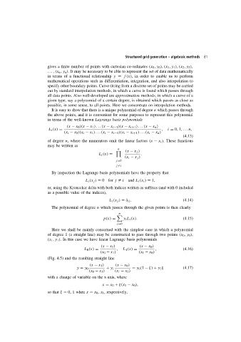
in terms of the well-known Lagrange basis polynomials
(x − x 0 )(x − x 1 ). ..(x − x i−1 )(x − x i+1 )...(x − x n )
L i (x) = , i = 0, 1,. ..n,
(x i − x 0 )(x i − x 1 )...(x i − x i−1 )(x i − x i+1 )...(x i − x n )
(4.13)
of degree n, where the numerators omit the linear factors (x − x i ). These functions
may be written as
n
(x − x j )

L i (x) = .
(x i − x j )
j=0
j =i
By inspection the Lagrange basis polynomials have the property that
L i (x j ) = 0for j = i and L i (x i ) = 1,
or, using the Kronecker delta with both indices written as suffixes (and with 0 included
as a possible value of the indices),
L i (x j ) = δ ij . (4.14)
The polynomial of degree n which passes through the given points is then clearly
n

p(x) = y i L i (x). (4.15)
i=0
Here we shall be mainly concerned with the simplest case in which a polynomial
of degree 1 (a straight line) may be constructed to pass through two points (x 0 ,y 0 ),
(x 1 ,y 1 ). In this case we have linear Lagrange basis polynomials
(x − x 1 ) (x − x 0 )
L 0 (x) = , L 1 (x) = , (4.16)
(x 0 − x 1 ) (x 1 − x 0 )
(Fig. 4.5) and the resulting straight line
(x − x 1 ) (x − x 0 )
y = y 0 + y 1 = y 0 (1 − ξ) + y 1 ξ (4.17)
(x 0 − x 1 ) (x 1 − x 0 )
with a change of variable on the x-axis, where
x = x 0 + ξ(x 1 − x 0 ),
so that ξ = 0, 1 when x = x 0 , x 1 , respectively.