Page 90 - Basic Structured Grid Generation

Structured grid generation – algebraic methods 79

a grid in the physical region where increments in r and θ (or ξ and η) along grid
lines θ = const. and grid curves r = const., respectively, are constant. This method of
generating a grid in the physical region, using a single analytical transformation (4.10)
or a combination of transformations (4.9) and (4.7), may be regarded as one form of
an algebraic method of grid generation.
Note, however, that eqns (4.9) are not the only way to transform the rectangle in
Fig. 4.3 into a unit square. Another one is given by the equations
ln(r/r 1 ) θ
ξ = , η = . (4.11)
ln(r 2 /r 1 ) α
It turns out that this transformation satisfies the requirements of one of the funda-
mental elliptic grid generation methods, as discussed in the first section of the next
chapter, namely that each of ξ, η satisfies Laplace’s equation (in two dimensions here):
2
2
∇ ξ = 0, ∇ η = 0.
A uniform grid in computational ξ, η space still maps to a grid in physical space, but
note now that equal increments in ξ do not correspond to equal increments in r.The
grid in physical space still consists of radial lines and concentric circles, but the distance
between the concentric circles diminishes as the inner boundary r = r 1 is approached.
If this is not regarded as a desirable feature of the grid, the spacing of grid lines can
be adjusted using an additional transformation with stretching functions as shown in
Section 4.4 below or through the use of control functions as described in Chapter 5.
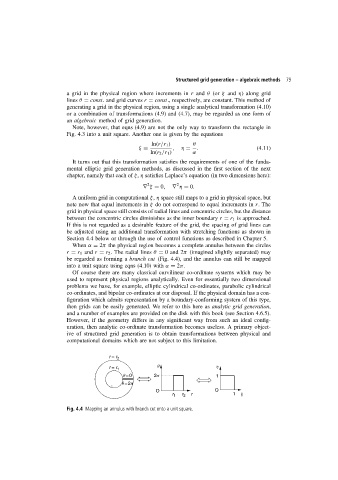
When α = 2π the physical region becomes a complete annulus between the circles
r = r 1 and r = r 2 . The radial lines θ = 0and 2π (imagined slightly separated) may
be regarded as forming a branch cut (Fig. 4.4), and the annulus can still be mapped
into a unit square using eqns (4.10) with α = 2π.
Of course there are many classical curvilinear co-ordinate systems which may be
used to represent physical regions analytically. Even for essentially two dimensional
problems we have, for example, elliptic cylindrical co-ordinates, parabolic cylindrical
co-ordinates, and bipolar co-ordinates at our disposal. If the physical domain has a con-
figuration which admits representation by a boundary-conforming system of this type,
then grids can be easily generated. We refer to this here as analytic grid generation,
and a number of examples are provided on the disk with this book (see Section 4.6.5).
However, if the geometry differs in any significant way from such an ideal config-
uration, then analytic co-ordinate transformation becomes useless. A primary object-
ive of structured grid generation is to obtain transformations between physical and
computational domains which are not subject to this limitation.

r = r 2
r = r 1 q h
q = 0 2p 1
q = 2p
O O
r 1 r 2 r 1 x

Fig. 4.4 Mapping an annulus with branch cut onto a unit square.