Page 88 - Basic Structured Grid Generation

Structured grid generation – algebraic methods 77

y

(j +1)k
i−1,j+1i,j+1 i+1,j+1
jk
i−1,j i,j i+1,j
(j −1)k
i−1,j−1i,j−1 i+1,j−1

O
(i−1)h ih (i+1)h x

Fig. 4.1 Rectangular array of points for finite differences.

and
2
∂ f 1
(f i+1,j+1 + f i−1,j−1 − f i+1,j−1 − f i−1,j+1 ), (4.6)
∂x∂y 4hk
all with second-order accuracy, as may be easily verified using Taylor Series expan-
sions. A variety of methods will generally be available to solve the resulting algebraic
equations for the grid-point values of the field quantities, provided that the boundary
or initial conditions can be incorporated in some way. However, this may not be an
easy task, particularly if the boundaries are not rectangular.
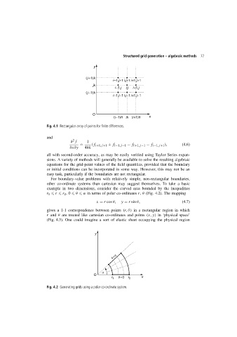
For boundary-value problems with relatively simple, non-rectangular boundaries,
other co-ordinate systems than cartesian may suggest themselves. To take a basic
example in two dimensions, consider the curved area bounded by the inequalities
r 1 r r 2 ,0 θ α in terms of polar co-ordinates r, θ (Fig. 4.2). The mapping
x = r cos θ, y = r sin θ, (4.7)

gives a 1-1 correspondence between points (r, θ) in a rectangular region in which
r and θ are treated like cartesian co-ordinates and points (x, y) in ‘physical space’
(Fig. 4.3). One could imagine a sort of elastic sheet occupying the physical region

y

q=a

a
O
r 1 q=0 r 2 x
Fig. 4.2 Generating grids using a polar co-ordinate system.