Page 93 - Basic Structured Grid Generation

82 Basic Structured Grid Generation

L (x) L (x)
1
0
1

0
x 0 x 1 x
Fig. 4.5 Linear Lagrange basis polynomials.

L (x) L (x) L (x)
0
2
1
1
0
x 0 x 1 x 2 x
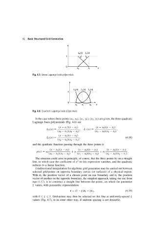
Fig. 4.6 Quadratic Lagrange basis polynomials.

In the case where three points (x 0 ,y 0 ), (x 1 ,y 1 ), (x 2 ,y 2 ) are given, the three quadratic
Lagrange basis polynomials (Fig. 4.6) are

(x − x 1 )(x − x 2 ) (x − x 0 )(x − x 2 )
L 0 (x) = , L 1 (x) = ,
(x 0 − x 1 )(x 0 − x 2 ) (x 1 − x 0 )(x 1 − x 2 )
(x − x 0 )(x − x 1 )
L 2 (x) = , (4.18)
(x 2 − x 0 )(x 2 − x 1 )
and the quadratic function passing through the three points is

(x − x 1 )(x − x 2 ) (x − x 0 )(x − x 2 ) (x − x 0 )(x − x 1 )
p(x) = y 0 + y 1 + y 2 .
(x 0 − x 1 )(x 0 − x 2 ) (x 1 − x 0 )(x 1 − x 2 ) (x 2 − x 0 )(x 2 − x 1 )
The situation could arise in principle, of course, that the three points lie on a straight
2
line, in which case the coefficient of x in this expression vanishes, and the quadratic
reduces to a linear function.
Unidirectional interpolation for algebraic grid generation may be carried out between
selected grid-points on opposite boundary curves (or surfaces) of a physical region.
With r 0 the position vector of a chosen point on one boundary and r 1 the position
vector of another on the opposite boundary, the simplest approach, taking our cue from
eqn (4.17), is to construct a straight line between the points, on which the parameter
ξ varies, with parametric representation
r = (1 − ξ)r 0 + ξr 1 , (4.19)

with 0 ξ 1. Grid-points may then be selected on this line at uniformly-spaced ξ
values (Fig. 4.7), or in some other way, if uniform spacing is not desirable.