Page 96 - Basic Structured Grid Generation

Structured grid generation – algebraic methods 85

4.2.2 Hermite interpolation polynomials

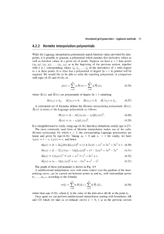
While the Lagrange interpolation polynomials match function values provided by data-
points, it is possible to generate a polynomial which matches first derivative values as
well as function values at a given set of points. Suppose we have n + 1 data points
(x 0 ,y 0 ), (x 1 ,y 1 ), ... ,(x n ,y n ) as at the beginning of the previous section, together

with n + 1 corresponding values y ,y ,...,y of the derivatives of y with respect
0 1 n
to x at these points. It is clear that a polynomial of degree 2n + 1 in general will be
required. We would like to be able to write the matching polynomial, in comparison
with eqns (4.15) and (4.14), as
n n

˜
p(x) = y i H i (x) + y H i (x), (4.26)
i
i=0 i=0
where H i (x) and H i (x) are polynomials of degree 2n + 1 satisfying
˜

˜
˜
H i (x j ) = δ ij , H (x j ) = 0, H i (x j ) = 0, H i (x j ) = δ ij . (4.27)
i
A convenient set of formulas defines the Hermite interpolating polynomials H i (x),
˜
H i (x) in terms of the Lagrange polynomials as follows:
2

H i (x) ={1 − 2L (x i )(x − x i )}[L i (x)] , (4.28)
i
2
H i (x) = (x − x i )[L i (x)] . (4.29)
˜
It is straightforward to verify, using eqn (4.14), that these definitions satisfy eqn (4.27).
The most commonly used form of Hermite interpolation makes use of the cubic
Hermite polynomial,for which n = 1; the corresponding Lagrange polynomials are
linear and given by eqn (4.16). Taking x 0 = 0and x 1 = 1 for clarity, we have
L 0 (x) = 1 − x, L 1 (x) = x, and hence
3
2
2
2

H 0 (x) ={1 − 2L (0)x}[L 0 (x)] = (1 + 2x)(1 − x) = 2x − 3x + 1 (4.30)
0
2
2
2

H 1 (x) ={1 − 2L (1)(x − 1)}[L 1 (x)] = (3 − 2x)x = 3x − 2x 3 (4.31)
1
3
2
2
2
˜
H 0 (x) = x[L 0 (x)] = x(1 − x) = x − 2x + x (4.32)
3
2
2
2
˜
H 1 (x) = (x − 1)[L 1 (x)] = (x − 1)x = x − x . (4.33)
The graph of these polynomials is shown in Fig. 4.9
A unidirectional interpolation, now with some control over the gradient of the inter-
polating curve, can be carried out between points r 0 and r n , with intermediate points
r 1 ,.. . , r n−1 , according to the formula
n n

˜
r(ξ) = r i H i (ξ) + r H i (ξ) , (4.34)
i
i=0 i=0

rather than eqn (4.22), where r is the value of the derivative dr/dξ at the point r i .
i
Once again we can perform unidirectional interpolation starting with boundaries AB
and CD which we take as co-ordinate curves ξ = 0, 1 as in the previous section