Page 99 - Basic Structured Grid Generation

88 Basic Structured Grid Generation

f″ f″ i+1
i
y ″ i−1 y ″ i+1
y ″ i

t i t i+1

0
x i−1 x i x i+1 x
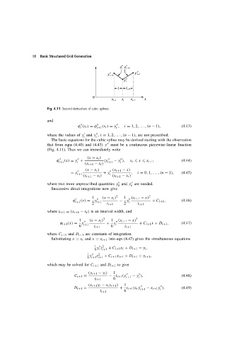
Fig. 4.11 Second derivatives of cubic splines.

and

φ (x i ) = φ (x i ) = y , i = 1, 2,. ..,(n − 1), (4.43)
i i+1 i

where the values of y and y , i = 1, 2,...,(n − 1), are not prescribed.
i i
The basic equations for the cubic spline may be derived starting with the observation

that from eqns (4.40) and (4.43) y must be a continuous piecewise-linear function
(Fig. 4.11). Thus we can immediately write
(x − x i )

φ (x) = y + (y − y ), (4.44)
i+1 i i+1 i x i x x i+1
(x i+1 − x i )
(x − x i ) (x i+1 − x)
= y i+1 + y , i = 0, 1,...,(n − 1), (4.45)
i
(x i+1 − x i ) (x i+1 − x i )
where two more unprescribed quantities y and y are needed.

0
n
Successive direct integrations now give
1 (x − x i ) 2 1 (x i+1 − x) 2

φ i+1 (x) = y i+1 − y i + C i+1 , (4.46)
2 t i+1 2 t i+1
where t i+1 = (x i+1 − x i ) is an interval width, and
1 (x − x i ) 3 1 (x i+1 − x) 3
φ i+1 (x) = y + y i + C i+1 x + D i+1 , (4.47)
i+1
6 t i+1 6 t i+1
where C i+1 and D i+1 are constants of integration.
Substituting x = x i and x = x i+1 into eqn (4.47) gives the simultaneous equations
1 2 + C i+1 x i + D i+1 = y i ,
y t
6 i i+1
1 t 2 + C i+1 x i+1 + D i+1 = y i+1 ,
y
6 i+1 i+1
which may be solved for C i+1 and D i+1 to give
(y i+1 − y i ) 1

C i+1 = − t i+1 (y i+1 − y ), (4.48)
i
t i+1 6
(x i+1 y i − x i y i+1 ) 1

D i+1 = + t i+1 (x i y i+1 − x i+1 y ). (4.49)
i
t i+1 6