Page 100 - Basic Structured Grid Generation

Structured grid generation – algebraic methods 89

Substituting into eqn (4.47), we obtain the basic equations of the cubic spline:

1 (x i+1 − x) 3 1 (x − x i ) 3
φ i+1 (x) = y i − t i+1 (x i+1 − x) + y i+1 − t i+1 (x − x i )
6 t i+1 6 t i+1
(x i+1 − x) (x − x i )
+y i + y i+1 , i = 0, 1,. ..,(n − 1). (4.50)
t i+1 t i+1

The second derivatives y , i = 0, 1,...,n, however, appear as undetermined quanti-
i
ties in these equations. To proceed further, we still have the continuity condition (4.42)
to apply. Equations (4.46) and (4.48) give
1 (x − x i ) 2 1 (x i+1 − x) 2 (y i+1 − y i ) 1

φ (x) = y − y + − t i+1 (y − y ).
i+1 i+1 i i+1 i
2 t i+1 2 t i+1 t i+1 6
(4.51)
Changing i to i − 1gives
1 (x − x i−1 ) 2 1 (x i − x) 2 (y i − y i−1 ) 1

φ (x) = y i − y i−1 + − t i (y − y i−1 ).
i
i
2 t i 2 t i t i 6
Consequently, eqn (4.42) gives
1 (y i+1 − y i ) 1 1 (y i − y i−1 ) 1

− y t i+1 + − t i+1 (y i+1 − y ) = y t i + − t i (y − y i−1 ),
i
i
i
i
2 t i+1 6 2 t i 6
which may be written as
(y i+1 − y i ) (y i − y i−1 )

t
y i−1 i + 2y (t i + t i+1 ) + y i+1 i+1 = 6 − ,
t
i
t i+1 t i
i = 1, 2,..., (n − 1) . (4.52)

Here we have a set of (n−1) linear equations for the (n+1) quantities y , so clearly
i
there is still some indeterminacy in the system. To resolve the problem we need to
specify two more conditions. There are a number of standard ways of doing this.

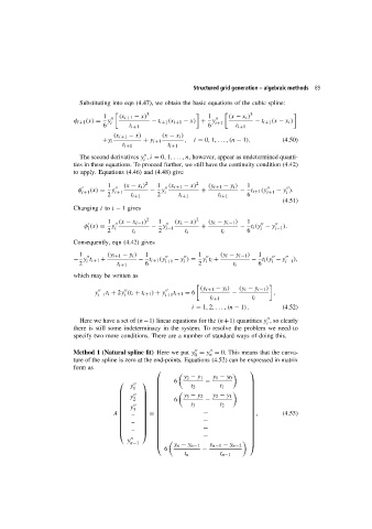
Method 1 (Natural spline fit) Here we put y = y = 0. This means that the curva-
0 n
ture of the spline is zero at the end-points. Equations (4.52) can be expressed in matrix
form as
 

y 2 − y 1 y 1 − y 0
6 −
   
y  t 2 t 1 
1
 

   
 y y 3 − y 2 y 2 − y 1
2   6 − 
   t 3 t 2 
 y 3   




A  –  =  −  , (4.53)
   
–
   − 
   
 –   − 
   
−
 

y n−1  
 y n − y n−1 y n−1 − y n−2 
6 −
t n t n−1