Page 97 - Basic Structured Grid Generation

86 Basic Structured Grid Generation

H (x) H (x)
0
1
1
∼
H (x)
0
0
1 x
∼
H (x)
1
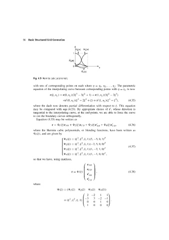
Fig. 4.9 Hermite cubic polynomials.

with sets of corresponding points on each where η = η 1 , η 2 ,. ..,η ˜ . The parametric
equation of the interpolating curve between corresponding points with η = η j is now
2
2
3
3
r(ξ, η j ) = r(0,η j )(2ξ − 3ξ + 1) + r(1,η j )(3ξ − 2ξ )
2
3
3
2

+r (0,η j )(ξ − 2ξ + ξ) + r (1,η j )(ξ − ξ ), (4.35)
where the dash now denotes partial differentiation with respect to ξ. This equation

may be compared with eqn (4.23). By appropriate choice of r , whose direction is
tangential to the interpolating curve, at the end-points, we are able to force the curve
to cut the boundary curves orthogonally.
Equation (4.35) may be written as
r = 1 (ξ)r AB + 2 (ξ)r CD + 3 (ξ)r AB + 4 (ξ)r CD , (4.36)
where the Hermite cubic polynomials, or blending functions, have been written as
i (ξ), and are given by
 3 2 T
1 (ξ) = (ξ ,ξ ,ξ, 1)(2, −3, 0, 1)



 3 2 T
 2 (ξ) = (ξ ,ξ ,ξ, 1)(−2, 3, 0, 0)
(4.37)
2
3
 3 (ξ) = (ξ ,ξ ,ξ, 1)(1, −2, 1, 0) T



4 (ξ) = (ξ ,ξ ,ξ, 1)(1, −1, 0, 0) ,
 3 2 T
so that we have, using matrices,
 
r AB
 
 r CD 
r = (ξ)   , (4.38)
 r 

AB 
r
CD
where
(ξ) = ( 1 (ξ) 2 (ξ) 3 (ξ) 4 (ξ))
 
2 −2 1 1
2
3
= (ξ ,ξ ,ξ, 1)  −3 3 −2 −1  .


 0 0 1 0 
1 0 0 0