Page 95 - Basic Structured Grid Generation

84 Basic Structured Grid Generation

h
h = 1 D
B 1
C x = 1
3
x = 0 A 3 C 2
A 2 C 1
A 1 C 0 1 x
A h = 0

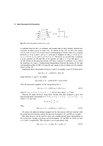
Fig. 4.8 Linear interpolation between two curves.

co-ordinate lines for the η co-ordinate, and assume that we have already selected sets
of points on these curves in some way. As shown in Fig. 4.8, we have five points
AA 1 A 2 A 3 B, CC 1 C 2 C 3 D on each curve corresponding to certain values of η, varying
between η = 0 at A and C and η = 1 at B and D. Suppose we take η = 0.25 at A 1 ,
C 1 , η = 0.5at A 2 , C 2 ,and η = 0.75 at A 3 , C 3 . Moreover we can take the co-ordinate
ξ to be constant on AB and CD; to be specific, we take ξ = 0on ABand ξ = 1
on CD. Points in the physical domain will have cartesian co-ordinates (x, y) which
are functions of ξ and η. Unidirectional interpolation between the points on AC and
corresponding points on BD will map the unit square in the ξη plane onto the domain
showninFig.4.8.
Employing linear interpolation between A and C according to eqn (4.19) then gives

r(ξ, 0) = (1 − ξ)r(0, 0) + ξr(1, 0),

while between A 1 and C 1 we obtain

r(ξ, 0.25) = (1 − ξ)r(0, 0.25) + ξr(1, 0.25).
Thus the parametric equation of the interpolating line is

r(ξ, η j ) = (1 − ξ)r(0,η j ) + ξr(1,η j ), (4.23)

j−1


where 0 η j = 1, j = 1, 2,... , ˜, and we have taken ˜ = 5here.
˜ −1
Marking off equal divisions along these straight lines then produces a grid. The
general grid-point corresponds to ξ = ξ i , η = η j , i = 1, 2,..., ˜ı, j = 1, 2,..., ˜,
ı
where ˜ = 5alsoand
i − 1
0 ξ i = 1.
˜ ı − 1
Thus
r(ξ i ,η j ) = (1 − ξ i )r(0,η j ) + ξ i r(1,η j ). (4.24)
Of course, the physical domain mapped out by this process will not coincide with
the actual physical domain, unless the physical boundaries AC and BD are straight.
The same process can be used to carry out a unidirectional linear interpolation in
the η-direction, starting with given curved boundaries AC and BD on which we take
η = 0 and 1, respectively. This will give a set of grid-points with

r(ξ i ,η j ) = (1 − η j )r(ξ i , 0) + η j r(ξ i , 1). (4.25)