Page 104 - Basic Structured Grid Generation

Structured grid generation – algebraic methods 93

h y

1 D
B
C
0 A
1 x O
x
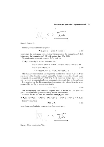
Fig. 4.13 Projector P η .

Similarly we can define the projector
P η (ξ, η) = (1 − η)r(ξ, 0) + ηr(ξ, 1) (4.68)
which maps the unit square onto a region which preserves the boundaries AC, BD,
but replaces the boundaries AB, CD with straight lines (Fig. 4.13).
We can form the composite mapping P ξ P η , such that
P ξ (P η (ξ, η)) = P ξ ((1 − η)r(ξ, 0) + ηr(ξ, 1))

= (1 − ξ)[(1 − η)r(0, 0) + ηr(0, 1)]+ ξ[(1 − η)r(1, 0) + ηr(1, 1)]
= (1 − ξ)(1 − η)r(0, 0) (4.69)
+(1 − ξ)ηr(0, 1) + ξ(1 − η)r(1, 0) + ξηr(1, 1).
This bilinear transformation has the property that the four vertices A, B, C, D are
preserved, but the boundaries are all replaced by straight lines; that is, the unit square
is mapped onto a quadrilateral ABDC (Fig. 4.14). Moreover, straight lines ξ = const.
and η = const. in computational space are mapped onto straight lines in physical space.
It is easy to show that this composition of projectors, often referred to as the tensor
productof P ξ and P η , is commutative; that is,
P ξ P η = P η P ξ . (4.70)
The accompanying disk contains a program, listed in Section 4.6.3, to generate a
grid in a straight-sided quadrilateral using bilinear transformation.
Note also that we can form the composite map P ξ P ξ ; we obtain

P ξ (P ξ (ξ, η)) = P ξ [(1 − ξ)r(0,η) + ξr(1,η)]= (1 − ξ)r(0,η) + ξr(1,η) = P ξ (ξ, η).
Hence we can write
P ξ P ξ = P ξ , (4.71)
which is the usual defining property of projection operators.

h y
1 D
B
C
0 A
1 x O
x
Fig. 4.14 Bilinear transformation P ξ P η .