Page 109 - Basic Structured Grid Generation

98 Basic Structured Grid Generation

From the above discussion it is clear that, in terms of projectors, the product P ξ P η P ς
is ‘algebraically minimal’, in that it is the weakest member of the set of projectors
to generate a grid (based on TFI) in R, given that it interpolates only from the eight
vertices of R. The Boolean sum P ξ ⊕P η ⊕P ς , on the other hand, is ‘algebraically maxi-
mal’ and the strongest member of the projector set. To use it we need boundary data on
all six faces of R (including the twelve edges and eight vertices). Then eqn (4.85) will
generate a grid within R by trilinear interpolation, taking discrete values of ξ, η, ς.
In practice, however, we may not have a complete set of boundary data. Suppose,
for example, that we have only boundary data pertaining to the twelve edges of the
physical region R. Since eqn (4.81) showed that the product P ξ P η interpolates linearly
from four edges of R, we might expect the appropriate grid generation formula to be
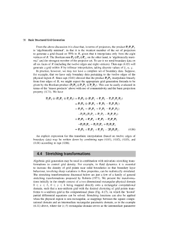
given by the Boolean product (P ξ P η ⊕ P η P ς ⊕ P ς P ξ ). This can be easily evaluated in
terms of the ‘tensor products’ above with use of commutativity and the basic projection
property (4.71). We have
P ξ P η ⊕ (P η P ς ⊕ P ς P ξ ) = P ξ P η ⊕ (P η P ς + P ς P ξ − P η P ς P ς P ξ )

= P ξ P η ⊕ (P η P ς + P ς P ξ − P η P ς P ξ )
= P ξ P η + (P η P ς + P ς P ξ − P η P ς P ξ )
−P ξ P η (P η P ς + P ς P ξ − P η P ς P ξ )

= P ξ P η + P η P ς + P ς P ξ − P η P ς P ξ
−P ξ P η P ς − P ξ P η P ς + P ξ P η P ς
= P ξ P η + P η P ς + P ς P ξ − 2P ξ P η P ς . (4.86)

An explicit expression for this transfinite interpolation (based on twelve edges of
boundary data) may be written down by combining eqns (4.81), (4.82), (4.83), and
(4.84) according to eqn (4.86).

4.4 Stretching transformations

Algebraic grid generation may be used in combination with univariate stretching trans-
formations to control grid density. For example, in fluid dynamics it is essential
to increase the density of grid points near solid boundaries so that boundary layer
behaviour, involving sharp variations in flow properties, can be realistically simulated.
The stretching transformations discussed below are just a few of a family of general
stretching transformations proposed by Roberts (1971). We present the transforma-
tions initially in the simple context of a two-dimensional rectangular physical domain
0 x L,0 y h being mapped directly onto a rectangular computational
domain, such that a non-uniform grid with the desired clustering of grid points trans-
forms to a uniform grid in the computational plane (Fig. 4.17), on which the ‘hosted’
partial differential equations can be solved. Stretching functions can also be applied
when the physical region is non-rectangular, as mappings between the square compu-
tational domain and an intermediate rectangular parametric domain, as in the example
(4.11) above, where the (r, θ) rectangular domain serves as the intermediate parameter