Page 111 - Basic Structured Grid Generation

100 Basic Structured Grid Generation

Note that we still have the boundary y = h mapping into the boundary η = 1. But
the boundary y = 0mapsto

ln{[β − 2α]/[β + 2α]}
η = α + (1 − α) ,
ln[(β + 1)/(β − 1)]
so the computational domain is not in general the same rectangle as in the previous
1
example, except for the case when α = . The variation of grid spacing in the y-
2
1
direction is again governed by the derivative dη/dy, which with α = is given by
2
dη 2β
= ,
dy 2y 2
2
h β − − 1 ln[(β + 1)/(β − 1)]
h
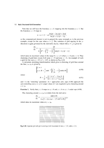
which takes its maximum values in the range 0 y h when y = 0and y = h. Thus
clustering of grid lines occurs both near y = 0 and near y = h. An example of such
a grid for the case α = 0.5, β = 1.07, is shown in Fig. 4.18.
A univariate stretching transformation which gives a clustering of grid lines around
the line y = y 0 is given by

ξ = x
1 −1 y (4.90)
η = B + sinh − 1 sinh(rB)
r y 0
where r
1 1 + (e − 1)y 0 /h
B = ln (4.91)
2r 1 − (1 − e −r )y 0 /h
and r is the ‘stretching’ parameter. As r approaches zero, eqns (4.90) approach the
zero-stretching case η = y/h. Larger values of r are required to give clustering around
y = y 0 .
Exercise 1. Verify that y = 0mapsto η = 0and y = h to η = 1 under eqn (4.90).

The clustering around y = y 0 is evident from the derivative
dη sinh (rB)
= .
dy ry 0 1 +[(y/y 0 ) − 1] sinh (rB) 1/2
2
2

which takes its maximum value at y = y 0 .

Fig. 4.18 Algebraic grid with grid clustering at both boundaries for beta = 1.07, alpha = 0.5.