Page 106 - Basic Structured Grid Generation

Structured grid generation – algebraic methods 95

h
1 y r t (x)
D
B r r (h)
r l (h)
0
1 x C
A r b (x)
O
x
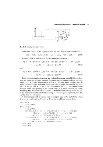
Fig. 4.15 Mapping of boundary curves.

At the four vertices of the physical domain we need the consistency conditions

r b (0) = r l (0), r b (1) = r r (0), r r (1) = r t (1), r l (1) = r t (0). (4.75)
Equation (4.74) is equivalent to the two component equations

x(ξ.η) = (1 − ξ)x l (η) + ξx r (η) + (1 − η)x b (ξ) + ηx t (ξ) − (1 − ξ)(1 − η)x b (0)
−(1 − ξ)ηx t (0) − (1 − η)ξx b (1) − ξηx t (1) (4.76)
and

y(ξ.η) = (1 − ξ)y l (η) + ξy r (η) + (1 − η)y b (ξ) + ηy t (ξ) − (1 − ξ)(1 − η)y b (0)
−(1 − ξ)ηy t (0) − (1 − η)ξy b (1) − ξηy t (1). (4.77)
These equations can be discretized and evaluated through a ‘nested DO loop’. Sup-
pose we choose (m + 1) grid nodes on the bottom and top boundaries in the computa-
tional plane, with equal increments
ξ = 1/m in ξ between nodes; similarly, (n + 1)
nodes on left and right, with equal increments
η = 1/n in η. We need the boundary
data for the functions r b , r t , r l , r r , i.e. the values of the (x, y) co-ordinates at the
selected points corresponding to the chosen values of ξ and η on each part of the
boundary. This data can be made available to the main routine through a data-file. Or,
if the boundaries can be calculated according to some analytical expression, then this
can be done in a subroutine.
A basic program with a ‘double loop’ to compute eqns (4.76) and (4.77), setting
ξ = s, η = t,
ξ = dX = 1/m,
η = dY = 1/n, would then take the form:

DO J=2,n
t=(J-1)*dY
DO 2 I=2,m
s=(I-1)*dX
X(I,J)=(1.0-s)*X l (J)+s*X r (J)+(1.0-t)*X b (I)+t*X t (I)
-(1.0-s)*(1.0-t)*X b (1)-(1.0-s)*t*X t (1)
-s*(1.0-t)*X b (m+1)-s*t*X t (m+1)
Y(I,J)=(1.0-s)*Y l (J)+s*Y r (J)+(1.0-t)*Y b (I)+t*Y t (I)
-(1.0-s)*(1.0-t)*Y b (1)-(1.0-s)*t*Y t (1)
-s*(1.0-t)*Y b (m+1)-s*t*Y t (m+1)
2 Continue
1 Continue