Page 113 - Basic Structured Grid Generation

102 Basic Structured Grid Generation

y
y=h (x)
2

y=h (x)
1
0
L x
Fig. 4.19 Divergent nozzle.

Here we extend the use of stretching functions to a non-rectangular physical domain.
Fig. 4.19 shows a two-dimensional divergent nozzle bounded by the curves y = h 1 (x)
and y = h 2 (x). The physical domain defined by 0 x L, h 1 (x) y h 2 (x) may
be mapped directly onto computational space 0 ξ, η 1 through

ξ = x
(4.98)
η =[y − h 1 (x)]/[h 2 (x) − h 1 (x)]
with inverse

x = ξ (4.99)
y = h 1 (ξ) +[h 2 (ξ) − h 1 (ξ)]η.
The accompanying disk contains a program for directly generating a grid using this
transformation, and is listed at Section 4.6.2.
We can concentrate the grid-lines near the boundaries by adapting eqn (4.97) in an
obvious way so that the mapping becomes (again with x = ξ)
 α
[h 2 (ξ) − h 1 (ξ)]η 1 (e αη/η 1 − 1)/(e − 1) + h 1 (ξ), 0 η η 1

y = [h 2 (ξ) − h 1 (ξ)][1 − (1 − η 1 ) (4.100)

× (e − 1)/(e − 1)]+ h 1 (ξ), η 1 η 1.
 α(1−η)/(1−η 1 ) α
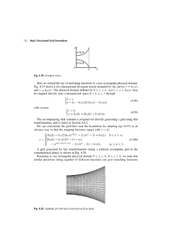
A grid generated by this transformation (using a uniform rectangular grid in the
computational plane) is shown in Fig. 4.20.
Returning to our rectangular physical domain 0 x L,0 y h, we note that
similar piecewise fitting together of Eriksson functions can give stretching functions

Fig. 4.20 Algebraic grid with grid-clustering near boundaries.