Page 89 - Basic Structured Grid Generation

78 Basic Structured Grid Generation

y
q
Computational plane
a

a
O
r 1 r 2 x
Physical plane O r 1 r 2 r

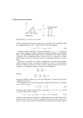
Fig. 4.3 Mapping a curved region onto a rectangle.

which is deformed by stretching, compression, and shearing into a rectangular shape
in ‘computational space’ (the r, θ plane) under the (inverse) mapping

2
2
r = x + y , θ = tan −1 (y/x). (4.8)
Boundary conditions specified on the curved boundaries r = r 1 , r = r 2 of physical
space are then mapped to boundary conditions on straight boundaries in computational
space, and a partial differential equation may be conveniently solved using a uniform
rectangular grid in computational space. Solution values at a grid-point in compu-
tational space may then be associated with the corresponding grid-point in physical
space.
The price to be paid for the geometric simplification is that the hosted equation,
initially expressed in terms of cartesian co-ordinates, has itself to be transformed to
the new co-ordinates, and this may result in a more complicated equation to solve. For
example, as is well-known, Laplace’s equation in two dimensions,
2
2
∂ ϕ ∂ ϕ
+ = 0
∂x 2 ∂y 2
becomes
2
2
∂ ϕ 1 ∂ϕ ∂ ϕ
+ + = 0
∂r 2 r ∂r ∂θ 2
in polar co-ordinates, which has an extra term, although it is clearly not much more
complicated in this case.
The mapping eqn (4.7) may be normalized by a further transformation of co-ordinates
from r, θ to ξ, η,where
r − r 1 θ
ξ = , η = , (4.9)
r 2 − r 1 α
which maps the rectangle in Fig. 4.3 into a unit square 0 ξ 1, 0 η 1inthe
ξ, η plane. Then eqns (4.7) become

x =[(r 2 − r 1 )ξ + r 1 ] cos(αη), y =[(r 2 − r 1 )ξ + r 1 ] sin(αη), (4.10)
which now maps a unit square in the new computational space onto the original curved
physical region. Moreover, a uniform rectangular grid in the unit square, where incre-
ments in ξ and η along grid lines between adjacent grid-points are constant, maps to