Page 128 - Basic Structured Grid Generation

Differential models for grid generation 117

y

O
x

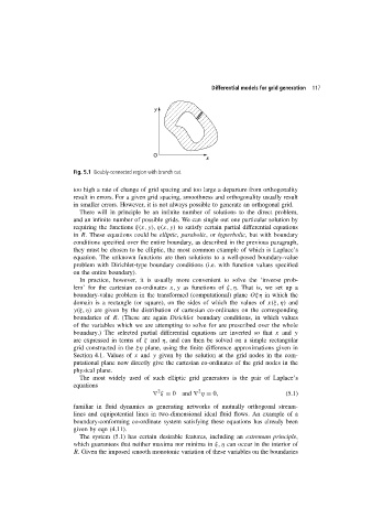
Fig. 5.1 Doubly-connected region with branch cut.

too high a rate of change of grid spacing and too large a departure from orthogonality
result in errors. For a given grid spacing, smoothness and orthogonality usually result
in smaller errors. However, it is not always possible to generate an orthogonal grid.
There will in principle be an infinite number of solutions to the direct problem,
and an infinite number of possible grids. We can single out one particular solution by
requiring the functions ξ(x, y), η(x, y) to satisfy certain partial differential equations
in R. These equations could be elliptic, parabolic,or hyperbolic, but with boundary
conditions specified over the entire boundary, as described in the previous paragraph,
they must be chosen to be elliptic, the most common example of which is Laplace’s
equation. The unknown functions are then solutions to a well-posed boundary-value
problem with Dirichlet-type boundary conditions (i.e. with function values specified
on the entire boundary).
In practice, however, it is usually more convenient to solve the ‘inverse prob-
lem’ for the cartesian co-ordinates x, y as functions of ξ, η. That is, we set up a
boundary-value problem in the transformed (computational) plane Oξη in which the
domain is a rectangle (or square), on the sides of which the values of x(ξ, η) and
y(ξ, η) are given by the distribution of cartesian co-ordinates on the corresponding
boundaries of R. (These are again Dirichlet boundary conditions, in which values
of the variables which we are attempting to solve for are prescribed over the whole
boundary.) The selected partial differential equations are inverted so that x and y
are expressed in terms of ξ and η, and can then be solved on a simple rectangular
grid constructed in the ξη plane, using the finite difference approximations given in
Section 4.1. Values of x and y given by the solution at the grid nodes in the com-
putational plane now directly give the cartesian co-ordinates of the grid nodes in the
physical plane.
The most widely used of such elliptic grid generators is the pair of Laplace’s
equations
2
2
∇ ξ = 0and ∇ η = 0, (5.1)
familiar in fluid dynamics as generating networks of mutually orthogonal stream-
lines and equipotential lines in two-dimensional ideal fluid flows. An example of a
boundary-conforming co-ordinate system satisfying these equations has already been
given by eqn (4.11).
The system (5.1) has certain desirable features, including an extremum principle,
which guarantees that neither maxima nor minima in ξ, η can occur in the interior of
R. Given the imposed smooth monotonic variation of these variables on the boundaries