Page 130 - Basic Structured Grid Generation

Differential models for grid generation 119

5.2 Control functions

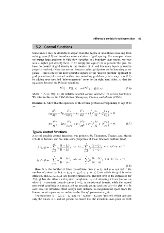
Sometimes it may be desirable to depart from the degree of smoothness resulting from
solving eqns (5.3) and introduce some variation of grid spacing. For example, where
we expect large gradients in fluid flow variables in a boundary-layer region, we may
seek a higher grid density there. If we simply use eqns (5.3) to generate the grid, we
have no control of grid density in the interior of R, and boundary layers cannot be
properly resolved. (Note that we can, however, select grid points on the boundary as we
please – this is one of the most desirable aspects of the ‘inverse problem’ approach to
grid generation.) A standard method for controlling grid density is to vary eqns (5.1)
by adding user-specified ‘inhomogeneous’ terms to the right-hand sides, so that the
equations become the Poisson equations
2
2
∇ ξ = P(ξ, η) and ∇ η = Q(ξ, η), (5.6)
where P(ξ, η), Q(ξ, η) are suitably selected control functions (or forcing functions).
We refer to this as the TTM Method (Thompson, Thames, and Mastin (1974)).

Exercise 1. Show that the equations of the inverse problem corresponding to eqn (5.6)
are
2
2
2
∂ x ∂ x ∂ x ∂x ∂x
g 22 2 − 2g 12 + g 11 2 + g P + Q = 0
∂ξ ∂ξ∂η ∂η ∂ξ ∂η
2
2
2
∂ y ∂ y ∂ y ∂y ∂y
g 22 2 − 2g 12 + g 11 2 + g P + Q = 0. (5.7)
∂ξ ∂ξ∂η ∂η ∂ξ ∂η
Typical control functions
A set of possible control functions was proposed by Thompson, Thames, and Mastin
(1974) as follows, and we state some properties of these functions without proof:
N I
2
2
(ξ − ξ n ) (ξ − ξ i ) −d i [(ξ−ξ i ) +(η−η i ) ] 2 1
P(ξ, η) =− a n e −c n |ξ−ξ n | − b i e
|ξ − ξ n | |ξ − ξ i |
n=1 i=1
N I
2
2
(η − η n ) (η − η i ) −d i [(ξ−ξ i ) +(η−η i ) ] 2 1
Q(ξ, η) =− a n e −c n |η−η n | − b i e .
|η − η n | |η − η i |
n=1 i=1
(5.8)
Here N is the number of lines (co-ordinate lines ξ = ξ n and η = η n )and I the
number of points (with ξ = ξ i ,η = η i ,0 ξ i ,η i 1) to which the grid is to be
attracted, and a n ,c n ,b i ,d i are positive parameters. The first term in the expression for
P(ξ, η) has the effect (with typical ‘amplitude’ a n ) of attracting ξ-lines (curves on
which ξ is constant) towards curves ξ = ξ n in the physical domain, while the second
term (with amplitude b i ) attracts ξ-lines towards points (and similarly for Q(ξ, η)). In
each case the attractive effect decays with distance in computational space from the
line or point in question according to the ‘decay’ parameters c n ,d i .
The functions (ξ − ξ n )/|ξ − ξ n | and (η − η n )/|η − η n | are functions which can take
only the values ±1, and are present to ensure that the attraction takes place on both