Page 131 - Basic Structured Grid Generation

120 Basic Structured Grid Generation

sides of ξ n -lines and η n -lines and in the entire neighbourhood of points (ξ i ,η i ).Taking
the amplitudes to be negative turns the attractive effects into repulsive ones.

5.3 Univariate stretching functions

One straightforward way of controlling grid density in the physical domain is through
the use of stretching functions (several examples of which were given in Section 4.4),
combined with a differential model of grid generation. Suppose that the transformation
(x, y) → (χ, σ) takes the physical domain R in two dimensions onto the square
0 χ, σ 1in χσ-space, such that the co-ordinates χ, σ are boundary-conforming.
We regard the χσ-space as an intermediate parameter space. A further mapping
χ = f 1 (ξ), σ = f 2 (η), (5.9)

with f 1 (0) = f 2 (0) = 0, f 1 (1) = f 2 (1) = 1, where the functions f 1 and f 2 are
one–one and onto, will map a square in ξη-computational space onto the square in
parameter space. But a regularly-spaced rectangular grid in computational space will in
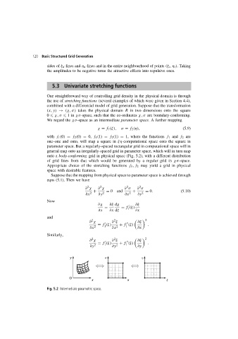
general map onto an irregularly-spaced grid in parameter space, which will in turn map
onto a body-conforming grid in physical space (Fig. 5.2), with a different distribution
of grid lines from that which would be generated by a regular grid in χσ-space.
Appropriate choice of the stretching functions f 1 ,f 2 may yield a grid in physical
space with desirable features.
Suppose that the mapping from physical space to parameter space is achieved through
eqns (5.1). Then we have

2
2
2
2
∂ χ ∂ χ ∂ σ ∂ σ
+ = 0and + = 0. (5.10)
∂x 2 ∂y 2 ∂x 2 ∂y 2
Now
∂χ ∂ξ dχ ∂ξ

= = f (ξ)
1
∂x ∂x dξ ∂x
and
2
2
∂ χ ∂ ξ ∂ξ 2

= f (ξ) + f (ξ) .
1
1
∂x 2 ∂x 2 ∂x
Similarly,
2
2
∂ χ ∂ ξ ∂ξ 2

= f (ξ) + f (ξ) .
1
1
∂y 2 ∂y 2 ∂y
y s h
O
x x x
Fig. 5.2 Intermediate parametric space.