Page 132 - Basics of MATLAB and Beyond

is numbered from top to bottom. The j axis is horizontal and is
numbered from left to right.

axis xy puts matlab into its default “Cartesian” axes mode. The coor-
dinate system origin is at the lower left corner. The x axis is hor-
izontal and is numbered from left to right. The y axis is vertical
and is numbered from bottom to top.
axis equal sets the aspect ratio so that equal tick mark increments on
the x-, y-, and z-axis are equal in size. This makes sphere(25)
look like a sphere, instead of an ellipsoid.
axis image is the same as axis equal except that the plot box fits
tightly around the data.
axis square makes the current axis box a square.
axis normal restores the current axis box to full size and removes any
restrictions on the scaling of the units. This undoes the effects of
axis square and axis equal.

axis off turns off all axis labeling (including the title), tick marks, and
background.

axis on turns axis labeling, tick marks and background back on.
axis vis3d prevents matlab from stretching the Axes to fit the size
of the Figure window or otherwise altering the proportions of the
objects as you change the 3-D viewing angle.

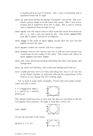
Let us look at some quick examples. Create sine and cosine compo-
nents and plot a circle:

t = linspace(0,2*pi);
x = cos(t);y = sin(t);
plot(x,y)

The default behaviour here is such that the data are stretched to fill the
rectangular Axes position. To make it look like a circle use:

axis equal

To get the top half of the circle:

axis([-1 1 0 1])

c 2000 by CRC Press LLC