Page 63 - Basics of MATLAB and Beyond

16 Polar Plots

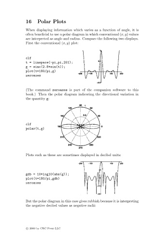
When displaying information which varies as a function of angle, it is
often beneficial to use a polar diagram in which conventional (x, y) values
are interpreted as angle and radius. Compare the following two displays.
First the conventional (x, y) plot:

clf
t = linspace(-pi,pi,201);
g = sinc(2.8*sin(t));
plot(t*180/pi,g)
zeroaxes

(The command zeroaxes is part of the companion software to this
book.) Then the polar diagram indicating the directional variation in
the quantity g:

clf
polar(t,g)

Plots such as these are sometimes displayed in decibel units:

gdb = 10*log10(abs(g));
plot(t*180/pi,gdb)
zeroaxes

But the polar diagram in this case gives rubbish because it is interpreting
the negative decibel values as negative radii:

c 2000 by CRC Press LLC