Page 104 - Becoming Metric Wise

94 Becoming Metric-Wise

2
is said to be χ -distributed (read: chi-square) with (m 2 1)(n 2 1) degrees
of freedom. This expression clearly is a sum of relative squared differ-
2
ences. It can be shown that the χ -distribution with k degrees of freedom
is the distribution of a sum of the squares of k independent standard nor-
mal variables explaining the meaning of the so-called “degrees of free-
dom”. If the expected frequencies can only be computed by estimating h
2
population parameters, we have a χ -distribution with (m 2 1)(n 2 1) 2 h
degrees of freedom. We omit the proofs.
If expected cell frequencies (not the observed ones!) are too small (in
practice ,6) we have to combine categories. For small tables it is recom-
mended to apply Yates corrections for continuity. This means that one
uses

m n 2 !
X X jO ij 2E ij j20:5
(4.24)
E ij
i51 j51
2
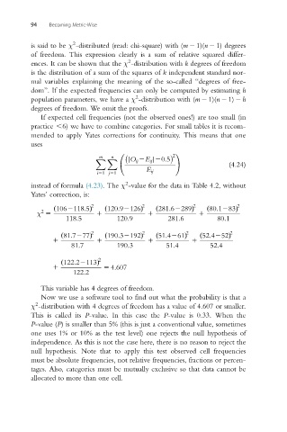
instead of formula (4.23). The χ -value for the data in Table 4.2, without
Yates’ correction, is:
2 2 2 2
ð 1062118:5Þ ð 120:92126Þ ð 281:62289Þ ð 80:1283Þ
2
χ 5 1 1 1
118:5 120:9 281:6 80:1
2 2 2 2
ð 81:7277Þ ð 190:32192Þ ð 51:4261Þ ð 52:4252Þ
1 1 1 1
81:7 190:3 51:4 52:4
2
ð 122:22113Þ
1 5 4:607
122:2

This variable has 4 degrees of freedom.
Now we use a software tool to find out what the probability is that a
2
χ -distribution with 4 degrees of freedom has a value of 4.607 or smaller.
This is called its P-value. In this case the P-value is 0.33. When the
P-value (P) is smaller than 5% (this is just a conventional value, sometimes
one uses 1% or 10% as the test level) one rejects the null hypothesis of
independence. As this is not the case here, there is no reason to reject the
null hypothesis. Note that to apply this test observed cell frequencies
must be absolute frequencies, not relative frequencies, fractions or percen-
tages. Also, categories must be mutually exclusive so that data cannot be
allocated to more than one cell.