Page 253 - Biomedical Engineering and Design Handbook Volume 2, Applications

232 DIAGNOSTIC EQUIPMENT DESIGN

B Gz
z
y

B G1 B G2

z x

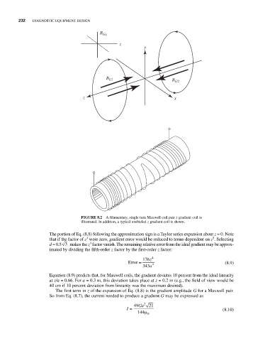
FIGURE 8.2 A filamentary, single turn Maxwell coil pair z gradient coil is
illustrated. In addition, a typical unshieled z gradient coil is shown.
The portion of Eq. (8.8) following the approximation sign is a Taylor series expansion about z = 0. Note
5
3
that if the factor of z were zero, gradient error would be reduced to terms dependent on z . Selecting
3
d = 0.5 3 makes the z factor vanish. The remaining relative error from the ideal gradient may be approx-
imated by dividing the fifth-order z factor by the first-order z factor:
176z 4
Error ≈ (8.9)
343a 4
Equation (8.9) predicts that, for Maxwell coils, the gradient deviates 10 percent from the ideal linearity
at z/a = 0.66. For a = 0.3 m, this deviation takes place at z = 0.2 m (e.g., the field of view would be
40 cm if 10 percent deviation from linearity was the maximum desired).
The first term in z of the expansion of Eq. (8.8) is the gradient amplitude G for a Maxwell pair.
So from Eq. (8.7), the current needed to produce a gradient G may be expressed as
49 Ga 2 21
I = (8.10)
144μ
0