Page 104 - Biosystems Engineering

Biosystems Analysis and Optimization 85

×
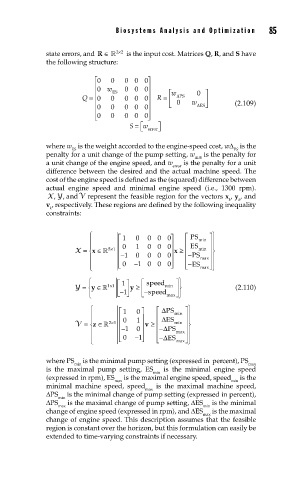
state errors, and R ∈ 22 is the input cost. Matrices Q, R, and S have
the following structure:

⎡0 0 000 ⎤
⎢ ⎥
⎢ 0 w ES 000 ⎥ ⎡ w 0 ⎤
⎢
Q = 0 0 000 ⎥ R R = ⎢ ΔPS w ⎥
0
⎢0 0 000 ⎥ ⎣ ΔES ⎦ (2.109)
⎢ ⎥
⎣ 0 0 000 ⎦
S = ⎡ ⎣ w error ⎤ ⎦
where w is the weight accorded to the engine-speed cost, wΔ is the
ES PS
penalty for a unit change of the pump setting, w is the penalty for
ΔES
a unit change of the engine speed, and w is the penalty for a unit
error
difference between the desired and the actual machine speed. The
cost of the engine speed is defined as the (squared) difference between
actual engine speed and minimal engine speed (i.e., 1300 rpm).
,
XY, and V represent the feasible region for the vectors x , y , and
k k
v , respectively. These regions are defined by the following inequality
k
constraints:
⎧ ⎤ ⎡ PS ⎤ ⎫ ⎫
⎪ ⎡ 1 0 000 ⎥ ⎢ min ⎥ ⎪
⎢
⎪
≥
×
X = x ⎨ ∈ 51 ⎢ 0 1 000 ⎥x ≥ ⎢ ES min ⎥ ⎪ ⎬
⎥
⎪ ⎢ −1 0 000 ⎥ − ⎢ PS max ⎪
⎥
⎪ ⎣ ⎢ 0 −1 000 ⎥ ⎦ ⎣ − ⎢ ES max ⎪
⎦ ⎭
⎩
⎧ ⎡ ⎤ ⎡ speed ⎤⎪ ⎫
⎪
1
×
Y = y ∈ 11 ⎢ ⎥ y ≥ ⎢ min ⎥⎬ (2.110)
⎨
−1
⎩ ⎪ ⎣ ⎦ ⎣ −speed max⎦ ⎭ ⎪
x
⎧ ⎤ ⎡ ΔPS ⎤ ⎫
⎪ ⎡ 1 0 ⎥ ⎢ min ⎥ ⎪
⎢
⎪
×
V = z ⎨ ∈ 21 ⎢ 0 1 ⎥ ≥ ⎢ ΔES min ⎥ ⎥ ⎪
⎬
v
⎪ ⎢ −1 0 ⎥ − ⎢ ΔPS max ⎥ ⎪
⎥
⎪ ⎣ ⎢ 0 −1⎥ ⎦ ⎦ ⎣ − ⎢ ΔES max ⎪
⎦ ⎭
⎩
where PS is the minimal pump setting (expressed in percent), PS
min max
is the maximal pump setting, ES is the minimal engine speed
min
(expressed in rpm), ES is the maximal engine speed, speed is the
max min
minimal machine speed, speed is the maximal machine speed,
max
ΔPS is the minimal change of pump setting (expressed in percent),
min
ΔPS is the maximal change of pump setting, ΔES is the minimal
max min
change of engine speed (expressed in rpm), and ΔES is the maximal
max
change of engine speed. This description assumes that the feasible
region is constant over the horizon, but this formulation can easily be
extended to time-varying constraints if necessary.