Page 103 - Biosystems Engineering

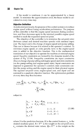
84 Chapter Two

If the model is nonlinear, it can be approximated by a linear
model. To minimize the approximation error, the linear model is cal-
culated in every time step.

Objective Definition
As indicated previously, the purpose of the control system is to reduce
engine speed without losing acceleration performance. The purpose
of this controller is that the engine speed increases during accelera-
tion, and then decreases again to the minimal possible engine speed
needed to reach the requested speed set point.
The objective of the controller is to minimize the set-point error
(between actual and desired machine speeds) with minimal input
cost. The input cost is the change of engine speed and pump setting.
This cost is chosen because it is related to the operator’s comfort. To
minimize engine speed, an extra penalty term in the engine-speed
state is added to the objective function. This is the mathematical
translation of our objective to operate the machine at minimal engine
speed. Equality constraints are formed by the dynamic model of the
system of Eq. (2.106). Inequality constraints are input constraints
(thus on change of pump setting and engine speed) and state constraints
(on the pump-setting and engine-speed state). Input constraints are
imposed to guarantee the operator’s comfort; state constraints con-
fine the pump setting and the engine speed to their physical region.
The squared set-point error, engine-speed cost, and input cost are
summed to a quadratic objective function. The optimization problem
at every time step thus becomes

N
N
) +
T
T
min ∑ (y − r ) S (y − r , y k ∑ (x − r ) Qx − r )
(
, k , y k k k x,,k k , x k
xy k ,u k k=1 k=1
k
M−1
+ ∑ vRv k (2.107)
T
k
k=0
subject to
x ⎧ = A x + B u
⎨ k+1 L k L k k = 0… N − 1
⎩ y k = C x + D v k
L k
L
⎧ x ∈X
⎪ k k = 1… N (2.108)
⎪
Y
⎨ y ∈Y k = 0… N − 1
k
⎪ k = 0… M − 1
⎪ ⎩ v ∈ V
k
where N is the prediction horizon, M is the control horizon, r is the
y,k
desired machine speed, S ∈ × 11 is the weight on the set-point error,
×
r contains the desired state values, Q ∈ 55 is the weight on the
x,k