Page 100 - Biosystems Engineering

Biosystems Analysis and Optimization 81

Controlled
current
Actual current
to the pump
Actual machine
X
speed
Actual engine
speed
Controlled
engine speed
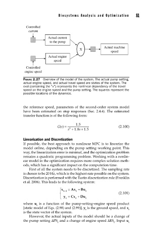
FIGURE 2.27 Overview of the model of the system. The actual pump setting,
actual engine speed, and actual travel speed are states of the system. The
oval (containing the "x") represents the nonlinear dependency of the travel
speed on the engine speed and the pump setting. The squares represent the
possible locations of the dynamics.

the reference speed, parameters of the second-order system model
have been estimated on step responses (Sec. 2.4.4). The estimated
transfer function is of the following form:

. 15
Gs() = (2.100)
2
.
.
s + 18 s + 15
Linearization and Discretization
If possible, the best approach to nonlinear MPC is to linearize the
model online, depending on the pump setting–working point. This
way, the linearization error is minimal, and the optimization problem
remains a quadratic programming problem. Working with a nonlin-
ear model in the optimization requires more complex solution meth-
ods, which has a significant impact on the computation time.
First of all the system needs to be discretized. The sampling rate
is chosen to be 20 Hz, which is the highest rate possible on the system.
Discretization is performed with the Tustin discretization rule (Franklin
et al. 2006). This leads to the following system:

⎪ x ⎧ k+1 = Ax + Bu k
k
⎨ (2.101)
⎪ y = Cx + Du k
⎩
k
k
where u is a function of the pump-setting–engine speed product
k
[static model of Eqs. (2.98) and (2.99)], y is the ground speed, and x
k k
is the state vector of the system.
However, the actual inputs of the model should be a change of
the pump setting ΔPS and a change of engine speed ΔES . Input u
k k k