Page 24 - Biosystems Engineering

Micr oarray Data Analysis Using Machine Learning Methods 5

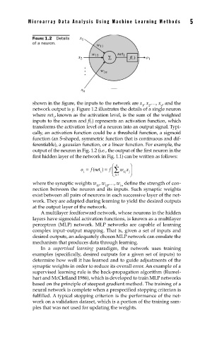
FIGURE 1.2 Details x 1
of a neuron. w 11

w 12 net 1
x 2 f(.) o 1

w 1n

x n

shown in the figure, the inputs to the network are x , x ,…, x , and the
1 2 n
network output is y. Figure 1.2 illustrates the details of a single neuron
where net , known as the activation level, is the sum of the weighted
1
inputs to the neuron and f(.) represents an activation function, which
transforms the activation level of a neuron into an output signal. Typi-
cally, an activation function could be a threshold function, a sigmoid
function (an S-shaped, symmetric function that is continuous and dif-
ferentiable), a gaussian function, or a linear function. For example, the
output of the neuron in Fig. 1.2 (i.e., the output of the first neuron in the
first hidden layer of the network in Fig. 1.1) can be written as follows:
⎛ n ⎞
o = f net =( ) f ⎜∑ w x j⎟
1 1 j 1 ⎠
⎝ =
j 1
where the synaptic weights w , w ,…, w define the strength of con-
11 12 1n
nection between the neuron and its inputs. Such synaptic weights
exist between all pairs of neurons in each successive layer of the net-
work. They are adapted during learning to yield the desired outputs
at the output layer of the network.
A multilayer feedforward network, whose neurons in the hidden
layers have sigmoidal activation functions, is known as a multilayer
perceptron (MLP) network. MLP networks are capable of learning
complex input–output mapping. That is, given a set of inputs and
desired outputs, an adequately chosen MLP network can emulate the
mechanism that produces data through learning.
In a supervised learning paradigm, the network uses training
examples (specifically, desired outputs for a given set of inputs) to
determine how well it has learned and to guide adjustments of the
synaptic weights in order to reduce its overall error. An example of a
supervised learning rule is the back-propagation algorithm (Rumel-
hart and McClelland 1986), which is developed to train MLP networks
based on the principle of steepest gradient method. The training of a
neural network is complete when a prespecified stopping criterion is
fulfilled. A typical stopping criterion is the performance of the net-
work on a validation dataset, which is a portion of the training sam-
ples that was not used for updating the weights.