Page 58 - Biosystems Engineering

Biosystems Analysis and Optimization 39

to the frequency content. Note that to avoid confusion between sig-
nals and systems represented in the time domain and their Laplace
transforms, the former are typically represented by lowercase letters
and the latter by uppercase letters.
Thanks to this transformation, we can convert signals and systems
from the time domain (function of time t) into the Laplace domain
(function of the Laplace operator s). This transformation has some
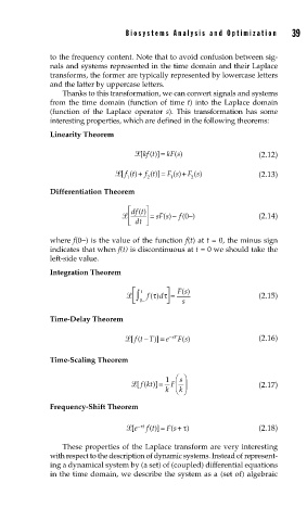
interesting properties, which are defined in the following theorems:

Linearity Theorem
=
t
[( )] kF ( ) (2.12)
kf
s
+
[ ( )+ f ( )] F () F () (2.13)
=
s
t
ft
s
1 2 1 2
Differentiation Theorem
⎡ df t() ⎤
⎢ ⎥ = sF s()− f( −0 ) (2.14)
⎣ dt ⎦
where f(0−) is the value of the function f(t)at t = 0, the minus sign
indicates that when f(t) is discontinuous at t = 0 we should take the
left-side value.
Integration Theorem
⎡ t ⎤ Fs()
τ
⎥
∫ ⎢ f() dτ = (2.15)
⎣ 0− ⎦ s
Time-Delay Theorem

[(ft T = − sT F ( ) (2.16)
−
)] e
s
Time-Scaling Theorem
s ⎛ ⎞
[( )] = 1 F ⎜ ⎟ (2.17)
t
fk
k ⎝ ⎠
k
Frequency-Shift Theorem
t =
[e −τ t f ( )] F + τ ) (2.18)
(s
These properties of the Laplace transform are very interesting
with respect to the description of dynamic systems. Instead of represent-
ing a dynamical system by (a set) of (coupled) differential equations
in the time domain, we describe the system as a (set of) algebraic