Page 61 - Biosystems Engineering

42 Chapter Two

m 2
f a (t)
x(t)
f a (t)

m 1 x 2 (t)

x (t)
1
k c

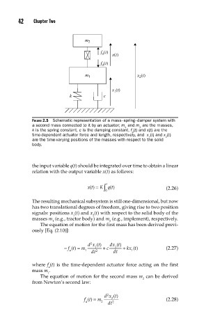
FIGURE 2.5 Schematic representation of a mass–spring–damper system with
a second mass connected to it by an actuator; m and m are the masses,
1 2
k is the spring constant, c is the damping constant, f (t) and x(t) are the
a
time-dependent actuator force and length, respectively, and x (t) and x (t)
1 2
are the time-varying positions of the masses with respect to the solid
body.

the input variable q(t) should be integrated over time to obtain a linear
relation with the output variable x(t) as follows:

∫
t
xt () = K q t () (2.26)
0
The resulting mechanical subsystem is still one-dimensional, but now
has two translational degrees of freedom, giving rise to two position
signals: positions x (t) and x (t) with respect to the solid body of the
1 2
masses m (e.g., tractor body) and m (e.g., implement), respectively.
1 2
The equation of motion for the first mass has been derived previ-
ously [Eq. (2.10)]:
2
dx t() dx t ()
1
1
− ft() = m + c + kx t () (2.27)
a 1 2 1
dt dt
where f (t) is the time-dependent actuator force acting on the first
a
mass m .
1
The equation of motion for the second mass m can be derived
2
from Newton’s second law:
2
dx t()
ft() = m 2 (2.28)
a 2 2
dt