Page 65 - Biosystems Engineering

46 Chapter Two

Time Delay or Dead Time
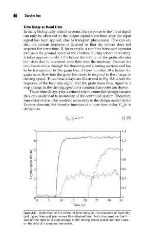
In many biologically related systems, the response to the input signal
can only be observed in the output signal some time after the input
signal has been applied, due to transport phenomena. One can say
that the system response is delayed or that the system does not
respond for some time. If, for example, a combine harvester operator
increases the ground speed of the combine during wheat harvesting,
it takes approximately 1.2 s before the torque on the grain elevator
belt rises due to increased crop flow into the machine. Because the
crop has to move through the threshing and cleaning sections and has
to be transported to the grain bin, it takes another 10 s before the
grain mass flow into the grain bin starts to respond to the change in
driving speed. These time delays are illustrated in Fig. 2.8 where the
response of the feed rate signal and the grain mass flow signal to a
step change in the driving speed of a combine harvester are shown.
These time delays play a critical role in controller design because
they can easily lead to instability of the controlled system. Therefore,
time delays have to be modeled accurately in the design model. In the
Laplace domain, the transfer function of a pure time delay G (s) is
td
defined as

G () = e −τ (2.35)
s
s
td
7 1.4

6 1.2

1
5
Ground speed (km/h) 4 0.8

0.6
3
2

0.2
1 0.4
0 0
0 5 10 15 20 25 30 35
Time (s)

FIGURE 2.8 Illustration of the effect of time delay in the response of feed rate
(solid grey line) and grain mass fl ow (dashed line), both displayed on the Y-
axis on the right on a step change in the driving speed (solid line and Y-axis
on the left) of a combine harvester.