Page 70 - Biosystems Engineering

Biosystems Analysis and Optimization 51

The magnitude and phase as functions of the frequency can thus be
derived from transfer function G(s) by replacing s with jω and deter-
mining the modulus and argument of G(jω), which, for any particular
frequency, is a complex number.

2.3.3 Bode Diagram of Transfer Functions
A system’s frequency response can be represented in several ways.
One of the most popular graphical representations is in a Bode dia-
gram that we treat in detail in this paragraph. A Bode diagram or
Bode plot of a transfer function is composed of two curves, a magni-
tude curve or plot, log(| (Gjω )|), drawn on a logarithmic scale and a
),
phase curve or plot, Gj( ω drawn on a linear scale. Both curves are
plotted against the frequency ω in radians per second, using a loga-
rithmic scale. The magnitude is most commonly plotted in decibels,
that is, 20log (| (Gjω )|).
10
We have shown that any transfer function G(s) can be factorized
into the form of Eq. (2.37). The factors in G(jω) can be written as vec-
tors in the complex s-plane in the following form:

s = j −ω p for i ∈[,1 n]
p i i
(2.52)
s = j −ω z for k ∈[,1 m]
z k
k
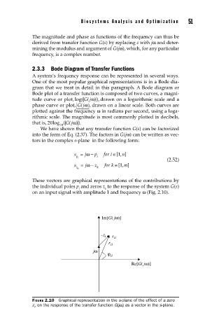
These vectors are graphical representations of the contributions by
the individual poles p and zeros z to the response of the system G(s)
i k
on an input signal with amplitude 1 and frequency ω (Fig. 2.10).

Im[G( j )]

–z i s zi
r zi
j
zi
Re[G( j )]

FIGURE 2.10 Graphical representation in the s-plane of the effect of a zero
z, on the response of the transfer function G(jω) as a vector in the s-plane.
i