Page 72 - Biosystems Engineering

Biosystems Analysis and Optimization 53

40
Magnitude (dB) –20
20
0

–40
10 –2 10 –1 10 0 10 1 10 2
100
50
Phase (°) 0

–50
–100
10 –2 10 –1 10 0 10 1 10 2
Frequency (rad/s)
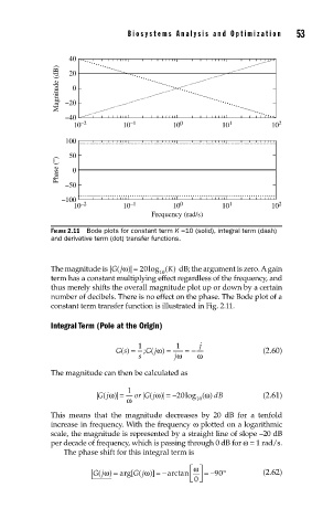
FIGURE 2.11 Bode plots for constant term K =10 (solid), integral term (dash)
and derivative term (dot) transfer functions.

The magnitude is | (Gjω= 20 log ( ) dB; the argument is zero. A gain
)|
K
10
term has a constant multiplying effect regardless of the frequency, and
thus merely shifts the overall magnitude plot up or down by a certain
number of decibels. There is no effect on the phase. The Bode plot of a
constant term transfer function is illustrated in Fig. 2.11.
Integral Term (Pole at the Origin)

ω
Gs() = 1 ; Gj ) = 1 = − j (2.60)
(
s jω ω
The magnitude can then be calculated as

1
ω
|(Gjω )|= or |(Gjω )|= −20 log ( ) dB (2.61)
ω 10
This means that the magnitude decreases by 20 dB for a tenfold
increase in frequency. With the frequency ω plotted on a logarithmic
scale, the magnitude is represented by a straight line of slope –20 dB
per decade of frequency, which is passing through 0 dB for ω = 1 rad/s.
The phase shift for this integral term is

ω⎤
=
ω
ω
(
(
Gj ) arg[ Gj )] = − arctan ⎡ ⎢ ⎥ =−90 ° (2.62)
⎣ ⎦
0