Page 76 - Biosystems Engineering

Biosystems Analysis and Optimization 57

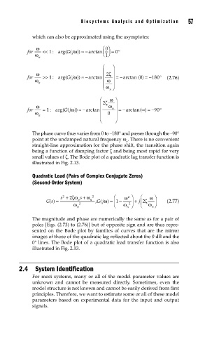
which can also be approximated using the asymptotes:

ω ⎛ ⎞ 0
G jω ≈ −arctan
for << 1 : arg( ( )) ⎜ ⎟ = 0°
ω ⎝ ⎠ 1
n
⎛ ⎞
ω ⎜ ζ 2 ⎟
−
for >> 1 : arg( Gj ( ω ≈ −arctan ⎜ ⎟ = −arctan ( )0 = −180° (2.76)
))
ω ω ⎜ ω ⎟
n
⎜ ⎝ ω ⎠ ⎟
n
⎛ 2ζ ω ⎞
ω ⎜ ω ⎟
1
n
for = :arg( (jω )) ≈ −arctan⎜ n ⎟ =− arctan( ) ∞ =− 90°
G
ω ⎜ 0 ⎟
n
⎜ ⎝ ⎟ ⎠
The phase curve thus varies from 0 to –180° and passes through the –90°
point at the undamped natural frequency ω . There is no convenient
n
straight-line approximation for the phase shift, the transition again
being a function of damping factor ζ and being most rapid for very
small values of ζ. The Bode plot of a quadratic lag transfer function is
illustrated in Fig. 2.13.
Quadratic Lead (Pairs of Complex Conjugate Zeros)
(Second-Order System)

s + 2ζω s + ω 2 ⎛ ω 2 ⎞ ⎛ ω ⎞
2
Gs() = n n ; Gj ) = 1ω ⎜ − ⎟ + j 2ζ ⎟ (2.77)
ζ
(
⎜
ω 2 ⎝ ω n ⎠ ⎝ ω ⎠
2
n n
The magnitude and phase are numerically the same as for a pair of
poles [Eqs. (2.73) to (2.76)] but of opposite sign and are thus repre-
sented on the Bode plot by families of curves that are the mirror
images of those of the quadratic lag reflected about the 0 dB and the
0° lines. The Bode plot of a quadratic lead transfer function is also
illustrated in Fig. 2.13.

2.4 System Identification
For most systems, many or all of the model parameter values are
unknown and cannot be measured directly. Sometimes, even the
model structure is not known and cannot be easily derived from first
principles. Therefore, we want to estimate some or all of these model
parameters based on experimental data for the input and output
signals.