Page 74 - Biosystems Engineering

Biosystems Analysis and Optimization 55

which can also be approximated using the asymptotes:

⎛ ⎞ 0
G jω ≈ −arctan
for ωτ << 1: arg( ( )) ⎜ ⎟ = 0°
⎝ ⎠ 1
(2.70)
for ωτ >>> 1: arg( (Gjω )) ≈ −arctan ⎛ ⎞1
⎜ ⎟ =−90°
⎝ ⎠ 0
A linear approximation can thus also be used for phase, that is, 0°
for ω≤ 0.1/τ and –90° for ω≥ 10/τ and a linear variation in between.
The true curve is gently curving. The error between the real curve
and the linear approximation is zero at the break-point frequency
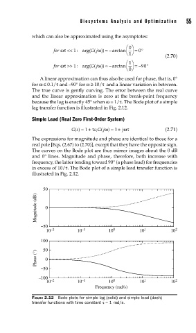
because the lag is exactly 45° when ω = 1/τ. The Bode plot of a simple
lag transfer function is illustrated in Fig. 2.12.

Simple Lead (Real Zero First-Order System)
ω
Gs() =+ τ sG j ) =+ jωτ (2.71)
(
;
1
1
The expressions for magnitude and phase are identical to those for a
real pole [Eqs. (2.67) to (2.70)], except that they have the opposite sign.
The curves on the Bode plot are thus mirror images about the 0 dB
and 0° lines. Magnitude and phase, therefore, both increase with
frequency, the latter tending toward 90° (a phase lead) for frequencies
in excess of 10/τ. The Bode plot of a simple lead transfer function is
illustrated in Fig. 2.12.

50
Magnitude (dB) 0

–50
10 –2 10 –1 10 0 10 1 10 2

100
Phase (°) 50 0

–50
–100
10 –2 10 –1 10 0 10 1 10 2
Frequency (rad/s)

FIGURE 2.12 Bode plots for simple lag (solid) and simple lead (dash)
transfer functions with time constant τ = 1 rad/s.