Page 79 - Biosystems Engineering

60 Chapter Two

1

0.5

Signal 0

–0.5

–1
0 10 20 30 40 50
Time (s)

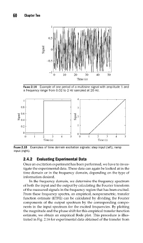
FIGURE 2.14 Example of one period of a multisine signal with amplitude 1 and
a frequency range from 0.02 to 2 Hz sampled at 20 Hz.

4
1
0.8 3
Signal 0.6 Signal 2
0.4
1
0.2
0 0
0 1 2 3 4 5 0 1 2 3 4 5
Time (s) Time (s)
FIGURE 2.15 Examples of time domain excitation signals: step input (left), ramp
input (right).
2.4.2 Evaluating Experimental Data
Once an excitation experiment has been performed, we have to inves-
tigate the experimental data. These data can again be looked at in the
time domain or in the frequency domain, depending on the type of
information desired.
In the frequency domain, we determine the frequency spectrum
of both the input and the output by calculating the Fourier transform
of the measured signals in the frequency region that has been excited.
From these frequency spectra, an empirical, nonparametric, transfer
function estimate (ETFE) can be calculated by dividing the Fourier
components of the output spectrum by the corresponding compo-
nents in the input spectrum for the excited frequencies. By plotting
the magnitude and the phase shift for this empirical transfer function
estimate, we obtain an empirical Bode plot. This procedure is illus-
trated in Fig. 2.16 for experimental data obtained of the transfer from