Page 84 - Biosystems Engineering

Biosystems Analysis and Optimization 65

In case we select a time domain model (when good prediction is
desired), parameters will be estimated by minimizing the deviation
of the simulated time response from the measured response. For this
purpose, the transfer function is redefined as a discrete time input–
output model. Because this model has both in the numerator and
denominator parameters to be estimated, a linear least squares opti-
mization is not the best option. Therefore, the parameter estimation is
typically done using the autoregressive moving average procedure
where the equation error term is described as a moving average of
white noise (Ljung 1987).
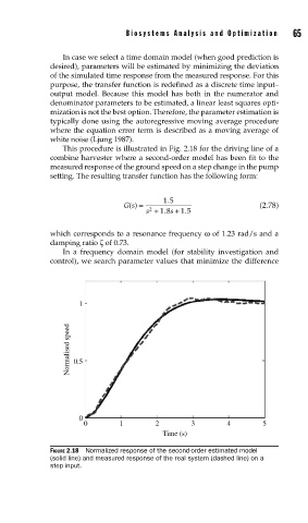
This procedure is illustrated in Fig. 2.18 for the driving line of a
combine harvester where a second-order model has been fit to the
measured response of the ground speed on a step change in the pump
setting. The resulting transfer function has the following form:

Gs() = . 15 (2.78)
2
.
s + 18 s + 15
.
which corresponds to a resonance frequency ω of 1.23 rad/s and a
damping ratio ζ of 0.73.
In a frequency domain model (for stability investigation and
control), we search parameter values that minimize the difference

1

Normalised speed 0.5

0
0 1 2 3 4 5
Time (s)

FIGURE 2.18 Normalized response of the second-order estimated model
(solid line) and measured response of the real system (dashed line) on a
step input.