Page 85 - Biosystems Engineering

66 Chapter Two

between the measured and the simulated frequency response func-
tion. This can be done using the least squares fitting procedure but
is more commonly performed using the nonlinear least squares pro-
cedure or a maximum likelihood procedure (Pintelon and Schoukens
2001). This procedure is illustrated for the depth control system of a
slurry injector for which the determination of the empirical transfer
function estimate has been described in this chapter (Sec. 2.3.2,
Fig. 2.16). For this system, a second-order model structure in the
numerator and a fourth-order model in the denominator has been
derived from first principles (Saeys et al. 2007). The parameters
of this model have been estimated by the nonlinear least squares
fitting procedure. This resulted in a transfer function in the following
form:

Ys () . 2 34 s + 6 .18 s + 663
2
Gs () = = (2.79)
3
2
4
Xs () s + 15 .1 s + 139s + 1560 s
s
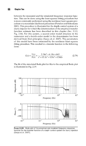
The fit of the simulated Bode plot for this to the empirical Bode plot
is illustrated in Fig. 2.19.

100
Magnitude (dB) 0

–100
10 –2 10 –1 10 0 10 1
Frequency (Hz)

0

Phase (°) –200

–400
10 –2 10 –1 10 0 10 1
Frequency (Hz)

FIGURE 2.19 Bode plot of the empirical and modeled frequency response
function for the transfer function of a depth control system for slurry injection
(Saeys et al. 2007).