Page 66 - Biosystems Engineering

Biosystems Analysis and Optimization 47

where τ is the time delay. Because this nonlinearity plays an impor-
tant role with respect to the stability of a controlled system, it is often
replaced by a linear approximation to be able to use linear stability
analysis tools such as root locus (Franklin et al. 2006). A useful linear
approximation is known as the second-order Padé approximant
(Franklin et al. 2006), presented by the following expression:

s − 6 s + 12
2
G () = e −τ ≈ τ τ 2 (2.36)
s
s
td 6 12
s + s +
2
τ τ 2
2.3 System Analysis
Once a design model is built, we want to investigate and predict the
system behavior under different conditions. For this purpose we can
make use of computer simulation tools.

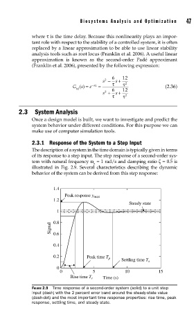
2.3.1 Response of the System to a Step Input
The description of a system in the time domain is typically given in terms
of its response to a step input. The step response of a second-order sys-
tem with natural frequency ω = 1 rad/s and damping ratio ζ = 0.5 is
n
illustrated in Fig. 2.9. Several characteristics describing the dynamic
behavior of the system can be derived from this step response:

1.4
Peak response y max
1.2
Steady state
1

Signal 0.8
0.6

0.4

0.2 Peak time T p
Settling time T s
0
0 5 10 15
Rise time T r Time (s)

FIGURE 2.9 Time response of a second-order system (solid) to a unit step
input (dash) with the 2 percent error band around the steady-state value
(dash-dot) and the most important time response properties: rise time, peak
response, settling time, and steady state.