Page 265 - Calculus Demystified

CHAPTER 8
252
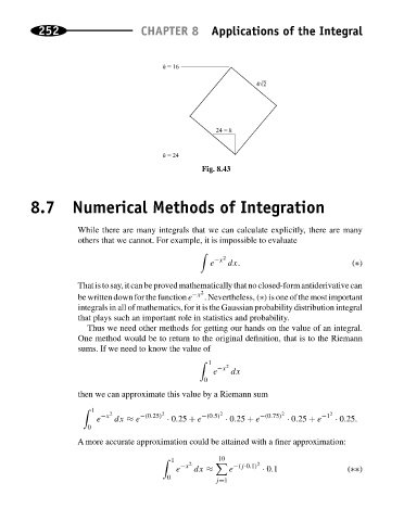
h = 16 Applications of the Integral
4√2

_
24 h

h = 24
Fig. 8.43

8.7 Numerical Methods of Integration

While there are many integrals that we can calculate explicitly, there are many
others that we cannot. For example, it is impossible to evaluate
2
e −x dx. (∗)

Thatistosay,itcanbeprovedmathematicallythatnoclosed-formantiderivativecan
be written down for the function e −x 2 . Nevertheless, (∗) is one of the most important
integrals in all of mathematics, for it is the Gaussian probability distribution integral
that plays such an important role in statistics and probability.
Thus we need other methods for getting our hands on the value of an integral.
One method would be to return to the original definition, that is to the Riemann
sums. If we need to know the value of
1 2
e −x dx
0
then we can approximate this value by a Riemann sum
1 2 2 2 2 2
e −x dx ≈ e −(0.25) · 0.25 + e −(0.5) · 0.25 + e −(0.75) · 0.25 + e −1 · 0.25.
0
A more accurate approximation could be attained with a finer approximation:

1 2 2
10
e −x dx ≈ e −(j·0.1) · 0.1 (∗∗)
0
j=1