Page 267 - Calculus Demystified

Applications of the Integral
CHAPTER 8
254
is made in this particular approximation. The rectangle gives rise to a “triangular”
error region (the difference between the true area under the curve and the area of the
rectangle). We put quotation marks around the word “triangular” since the region
in question is not a true triangle but instead is a sort of curvilinear triangle. If we
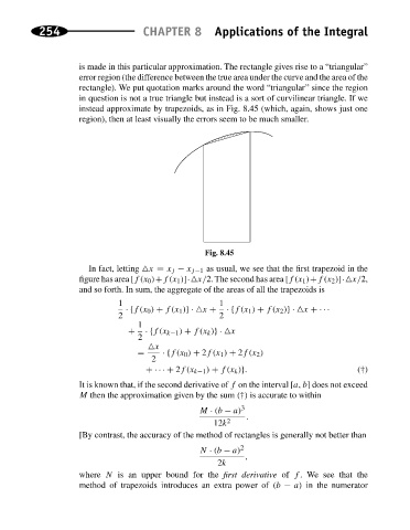
instead approximate by trapezoids, as in Fig. 8.45 (which, again, shows just one
region), then at least visually the errors seem to be much smaller.

Fig. 8.45

In fact, letting x = x j − x j−1 as usual, we see that the first trapezoid in the
figure has area [f(x 0 )+f(x 1 )]· x/2. The second has area [f(x 1 )+f(x 2 )]· x/2,
and so forth. In sum, the aggregate of the areas of all the trapezoids is
1 1
·{f(x 0 ) + f(x 1 )}· x + ·{f(x 1 ) + f(x 2 )}· x + ···
2 2
1
+ ·{f(x k−1 ) + f(x k )}· x
2
x
= ·{f(x 0 ) + 2f(x 1 ) + 2f(x 2 )
2
+ ··· + 2f(x k−1 ) + f(x k )}. (†)
It is known that, if the second derivative of f on the interval [a, b] does not exceed
M then the approximation given by the sum (†) is accurate to within
M · (b − a) 3
.
12k 2
[By contrast, the accuracy of the method of rectangles is generally not better than
N · (b − a) 2
,
2k
where N is an upper bound for the first derivative of f . We see that the
method of trapezoids introduces an extra power of (b − a) in the numerator