Page 266 - Calculus Demystified

CHAPTER 8
or Applications of the Integral 253
1 2 2
100
e −x dx ≈ e −(j·0.01) · 0.01 (.)
0
j=1
The trouble with these “numerical approximations” is that they are calcula-
tionally expensive: the degree of accuracy achieved compared to the number of
calculations required is not attractive.
Fortunately, there are more accurate and more rapidly converging methods for
calculating integrals with numerical techniques. We shall explore some of these in
the present section.
It should be noted, and it is nearly obvious to say so, that the techniques of
this section require the use of a computer. While the Riemann sum (∗∗) could be
computed by hand with some considerable effort, the Riemann sum (.) is all but
infeasible to do by hand. Many times one wishes to approximate an integral by the
sum of a thousand terms (if, perhaps, five decimal places of accuracy are needed).
In such an instance, use of a high-speed digital computer is virtually mandatory.

8.7.1 THE TRAPEZOID RULE

The method of using Riemann sums to approximate an integral is sometimes called
“the method of rectangles.” It is adequate, but it does not converge very quickly
and it begs more efficient methods. In this subsection we consider the method of
approximating by trapezoids.
Let f be a continuous function on an interval [a, b] and consider a partition
P ={x 0 ,x 1 ,...,x k } of the interval. As usual, we take x 0 = a and x k = b. We also
assume that the partition is uniform.

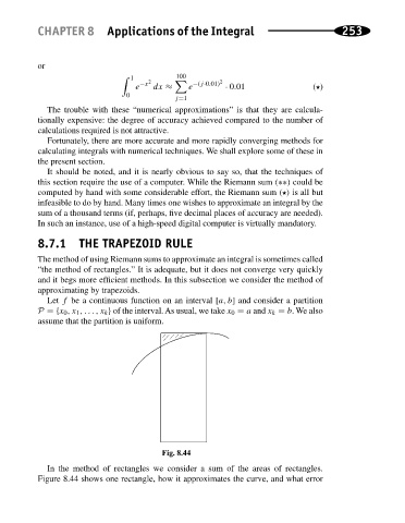
Fig. 8.44
In the method of rectangles we consider a sum of the areas of rectangles.
Figure 8.44 shows one rectangle, how it approximates the curve, and what error