Page 164 - Cam Design Handbook

THB5 8/15/03 1:53 PM Page 152

152 CAM DESIGN HANDBOOK

dS ∂ S df ∂ S ds
(
v f , ) = 1 = 1 2 + 1 2
s
1 2 2
dt ∂f dt ∂ s dt
2 2
∂ S ∂ S
= 1 w + 1 v
∂f 2 2 s ∂ 2 2
1 ()
= [ N f ()] ◊[]◊[ M s w +[ N f ()]◊[]◊[ M s ()] 1 () v (5.50)
()]
p
p
2 2 2 2 2 2
2 ( )
1 ()
A f , ) = [ N f ()] ◊[]◊[ M s w + 2[ N f ()] ◊[]◊[ M s ()] 1 () w v
(
()
]
2
p
s
p
1 2 2 2 2 2 2 2 22
+[ N f ()]◊[]◊[ M s ()] 2 () v 2 2 (5.51)
p
2
2
3 ()
2 ( )
(
]
J f , ) = [ N f ()] ◊[]◊[ M s w + 3[ N f ()] ◊[]◊[ M s ()] 1 ( ) w 2 2
()
p
v
3
2
s
p
2
2
2
2
2
2
1
2
1 ()
() 3
+ 3[ N f ()] ◊[]◊[ M s ()] 2 ( ) w v +[ N f ()]◊[]◊[ [ M s ()] v 3 (5.52)
p
p
2
2 2 22 2 2 2
i
th
i
where [N(f 2)] (I) =- [N(f 2)]/f 2 is the i order partial derivative. With respect to (f 2,
(j)
j
th
j
[M(s 2)]) = [M(s 2)], s 2 is the j order partial derivative, and with respect to s 2, w 2 = df 2/dt
is the angular velocity of the cam, and v 2= ds 2/dt is the linear velocity of the cam. Note
that the elements in the matrices above for the derivatives of B-splines in the rotating and
translating directions are found in Eqs. (5.43) to (5.46).
Example Application. The following numerical examples demonstrate the feasibility
of synthesizing the follower motions. In these two cases, a cam with a translating spheri-
cal follower is considered. The dimensional parameters used for the cam-follower mech-
anism in both examples are:
a = 22mm
l = 50mm
r = 5mm.
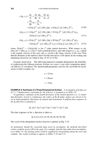
EXAMPLE 9: Synthesis of a Three-Dimensional Surface A rectangular grid data set
of 7 ¥ 7 displacement constraints for the follower is assumed as in Table 5.8.
To guarantee continuity of the fourth derivative of the motion function (i.e., to ensure
that derivative of jerk is continuous), the orders of the B-spline surface are chosen to be
six in both parametric directions of rotation and translation. A uniform knot sequence in
the f 2 direction is adopted as
, [
p
02p 7 4p 7 6p 7 8p 7 10p 7 12p 7 2 . ]
,
,
,
,
,
,
The knot sequence in the s 2 direction is taken as
[ 000000 25 50 50 50 50 50 50 . ]
,
,
,
,
,
,,,,,,
,
The result of the interpolated motion function is plotted in Fig. 5.34.
As mentioned, should the constraint data array be incomplete, the methods described
earlier could be used to fill in the gaps. For example, had the data table been incomplete,
as in Table 5.9, the missing points could be supplied by interpolating along the rows and
columns. The results of doing so appear in Tables 5.10 and 5.11.