Page 262 - Chiral Separation Techniques

240 9 Modeling and Simulation in SMB for Chiral Purification

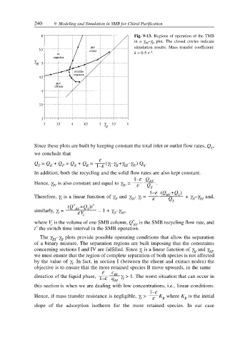
Fig. 9-13. Regions of operation of the TMB
in a γ –γ plot. The closed circles indicate
III II
simulation results. Mass transfer coefficient:
–1
k = 0.5 s .

Since these plots are built by keeping constant the total inlet or outlet flow rates, Q ,
T
we conclude that
ε
Q = Q + Q = Q + Q = (γ –γ +γ –γ ) Q .
T E F X R 1–ε I II III IV S
In addition, both the recycling and the solid flow rates are also kept constant.
1–ε Q
Hence, γ is also constant and equal to γ = ε RF .
IV IV Q S
1–ε (Q +Q )
Therefore, γ is a linear function of γ and γ : γ = RF T + γ –γ and,
I II III I ε Q II III
S
(Q * RF +Q )t *
T
similarly, γ = – 1 + γ –γ ,
I εV II III
c
where V is the volume of one SMB column, Q * RF is the SMB recycling flow rate, and
c
*
t the switch time interval in the SMB operation.
The γ –γ plots provide possible operating conditions that allow the separation
III II
of a binary mixture. The separation regions are built imposing that the constraints
concerning sections I and IV are fulfilled. Since γ is a linear function of γ and γ ,
I II III
we must ensure that the region of complete separation of both species is not affected
by the value of γ . In fact, in section I (between the eluent and extract nodes) the
I
objective is to ensure that the more retained species B move upwards, in the same
ε c
direction of the liquid phase, 1–ε q BI γ > 1. The worst situation that can occur in
I
BI
this section is when we are dealing with low concentrations, i.e., linear conditions.
1–ε
Hence, if mass transfer resistance is negligible, γ > K where K is the initial
I ε B B
slope of the adsorption isotherm for the more retained species. In our case