Page 113 - Circuit Analysis II with MATLAB Applications

Higher Order Delta Functions

vt vt
V
– t + 5
3

2 – t + 6

1
1 0 1 2 3 4 5 6 7

ts

1
2t
2

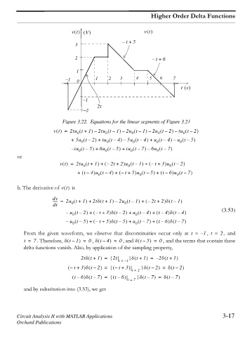
Figure 3.22. Equations for the linear segments of Figure 3.21
vt = 2tu t + 0 1 – 2tu t – 1 – 2u t – 1 – 2u t – 2 – tu t – 2

0
0
0
0

+ 5u t – 0 2 + tu t – 4 – 5u t – 4 + u t – 4 – u t – 5

0
0
0
0
tu t – – 0 5 + 6u t – 5 + tu t – 7 – 6u t – 7

0
0
0
or
vt = 2tu t + 0 1 + – 2t + 2 u t – 1 + – t + 3 u t – 2

0
0
+ t – 4 u t – 0 4 + – t + 5 u t – 5 + t – 6 u t – 7

0
0
b. The derivative of vt is
dv 2u t + 1 + 2tG t + 1 – 2u t – 1 + – 2t + 2 G t – 1
------ =

dt 0 0
(3.53)
u t – – 0 2 + – t + 3 G t – 2 + u t – 4 + t – 4 G t – 4

0
u t – – 0 5 + – t + 5 G t – 5 + u t – 7 + t – 6 G t – 7

0
From the given waveform, we observe that discontinuities occur only at t = – 1 , t = 2 , and
t = 7 . Therefore, G t – 1 = 0 , G t – 4 = 0 , and G t – 5 = 0 , and the terms that contain these

delta functions vanish. Also, by application of the sampling property,
–
2tG t + 1 = ^ 2t ` G t + 1 = 2G t + 1

t = – 1

– t + 3 G t – 2 = – t + 3 ^ ` G t – 2 = G t – 2

t = 2

t – 6 G t – 7 = t – 6 ^ ` G t – 7 = G t – 7

t = 7
and by substitution into (3.53), we get
Circuit Analysis II with MATLAB Applications 3-17
Orchard Publications