Page 114 - Circuit Analysis II with MATLAB Applications

Chapter 3 Elementary Signals

dv 2u t + 1 – 2G t + 1 – 2u t – 1 – u t – 2
------ =

dt 0 0 0 (3.54)
+
G t – 2 + u t – 0 4 – u t – 5 + u t – 7 + G t – 7

0
0
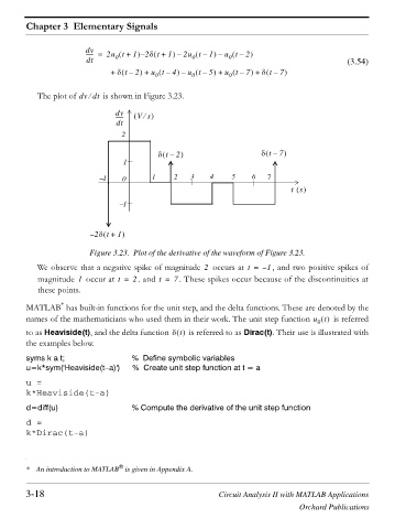
The plot of dv dte is shown in Figure 3.23.
dv
e
------ Vs
dt
2

G t – 2 G t – 7

1
1 0 1 2 3 4 5 6 7
ts
1
2G t + 1
–
Figure 3.23. Plot of the derivative of the waveform of Figure 3.23.

We observe that a negative spike of magnitude occurs at t = – 1 , and two positive spikes of
2
magnitude occur at t = 2 , and t = 7 . These spikes occur because of the discontinuities at
1
these points.
*
MATLAB has built-in functions for the unit step, and the delta functions. These are denoted by the
names of the mathematicians who used them in their work. The unit step function u t is referred
0
to as Heaviside(t), and the delta function G t is referred to as Dirac(t). Their use is illustrated with
the examples below.
syms k a t; % Define symbolic variables
u=k*sym('Heaviside(t a)') % Create unit step function at t = a
u =
k*Heaviside(t-a)
d=diff(u) % Compute the derivative of the unit step function

d =
k*Dirac(t-a)

®
* An introduction to MATLAB is given in Appendix A.

3-18 Circuit Analysis II with MATLAB Applications

Orchard Publications