Page 16 - Circuit Analysis II with MATLAB Applications

Chapter 1 Second Order Circuits

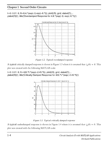
t=0: 0.01: 6; ft=8.4.*(exp( t)-exp( 6.*t)); plot(t,ft); grid; xlabel('t');...
ylabel('f(t)'); title('Overdamped Response for 4.8.*(exp( t) exp( 6.*t))')

Figure 1.2. Typical overdamped response

A typical critically damped response is shown in Figure 1.3 where it is assumed that i 0 = 0 . This
n
plot was created with the following MATLAB code:

t=0: 0.01: 6; ft=420.*t.*(exp( 2.45.*t)); plot(t,ft); grid; xlabel('t');...
ylabel('f(t)'); title('Critically Damped Response for 420.*t.*(exp( 2.45.*t))')

Figure 1.3. Typical critically damped response
A typical underdamped response is shown in Figure 1.4 where it is assumed that i 0 = 0 . This
n
plot was created with the following MATLAB code:

1-4 Circuit Analysis II with MATLAB Applications
Orchard Publications