Page 18 - Circuit Analysis II with MATLAB Applications

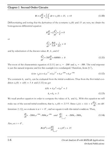
Chapter 1 Second Order Circuits

di 1 t
Ri + L----- + ---- ³ it + v 0 = 15 t ! 0 (1.10)
d
dt C 0 C
Differentiating and noting that the derivatives of the constants v 0 and 15 are zero, we obtain the
C
homogeneous differential equation

2
di d i i
R----- + L------- + ---- = 0
dt dt 2 C
or
2
d i Rdi i
------- + -------- + ------- = 0
dt 2 Ldt LC
and by substitution of the known values , , and C
RL
2
d i di
------- + 500----- + 60000i = 0 (1.11)
dt 2 dt
The roots of the characteristic equation of (1.11) are s = – 200 and s = – 300 . The total response
2
1
is just the natural response and for this example it is overdamped. Therefore, from (1.7),
s t s t – 200t – 300t
2
1
it = i t = k e + k e = k e + k e (1.12)
1
2
1
n
2
The constants and can be evaluated from the initial conditions. Thus from the first initial con-
k
k
1
2
dition i 0 = i0 = 5A and (1.12) we get
L
0
0
i0 = k e + k e = 5
1
2
k + k = 5 (1.13)
2
1
We need another equation in order to compute the values of k 1 and k 2 . With this equation we will
dv
C
make use of the second initial condition, that is, v 0 = 2.5 V . Since i t = it = C-------- , we dif-
C
C
dt
ferentiate (1.12), we evaluate it at t = 0 + , and we equate it with this initial condition. Then,
di – 200t – 300t di
–
-----= – 200k e – 300k e and ----- = – 200k 300k (1.14)
dt 1 2 dt 1 2
t = 0 +
Also, at t = 0 + ,
+ di +
Ri 0 + L----- v 0 + = 15
c
dt +
t = 0
1-6 Circuit Analysis II with MATLAB Applications
Orchard Publications