Page 20 - Circuit Analysis II with MATLAB Applications

Chapter 1 Second Order Circuits

1st derivative of solution is y1 =
-23000*exp(-200*t)+33000*exp(-300*t)

2nd derivative of solution is y2 =
4600000*exp(-200*t)-9900000*exp(-300*t)
Differential equation is satisfied since y = y2+y1+y0 = 0

1st initial condition is satisfied since at t = 0, i0 = 5

2nd initial condition is also satisfied since vC+vL+vR=15 and vC0
= 2.5000

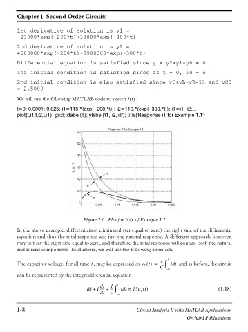
We will use the following MATLAB code to sketch it .

t=0: 0.0001: 0.025; i1=115.*(exp( 200.*t)); i2=110.*(exp( 300.*t)); iT=i1 i2;...
plot(t,i1,t,i2,t,iT); grid; xlabel('t'); ylabel('i1, i2, iT'); title('Response iT for Example 1.1')

Figure 1.6. Plot for it of Example 1.1

In the above example, differentiation eliminated (set equal to zero) the right side of the differential
equation and thus the total response was just the natural response. A different approach however,
may not set the right side equal to zero, and therefore the total response will contain both the natural
and forced components. To illustrate, we will use the following approach.

1 t
t
d
The capacitor voltage, for all time , may be expressed as v t = ---- ³ it and as before, the circuit
C
C
– f
can be represented by the integrodifferential equation
di 1 t
Ri + L----- + ---- ³ it = 15u t (1.18)
d
dt C 0
– f
1-8 Circuit Analysis II with MATLAB Applications
Orchard Publications