Page 24 - Circuit Analysis II with MATLAB Applications

Chapter 1 Second Order Circuits

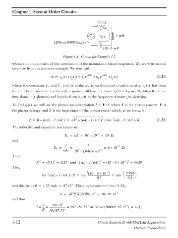
0.5 :

+ 1mH
it `
200cos 10000t u t V

0
100 6 mF
e
Figure 1.8. Circuit for Example 1.2
whose solution consists of the summation of the natural and forced responses. We know its natural
response from the previous example. We start with

it = i t + i t = k e – 200t + k e – 300t + i t (1.31)
f
n
f
2
1
where the constants k 1 and k 2 will be evaluated from the initial conditions after i t has been
f
found. The steady state (or forced) response will have the form i t = k cos 10 000t + T in the

f
3
t
time domain ( -domain) and has the form k ‘ T in the frequency domain (jZ -domain).
3
V
I
To find i t we will use the phasor analysis relation I = V Z where is the phasor current, is
e
f
the phasor voltage, and is the impedance of the phasor circuit which, as we know, is
Z
2
Z = R + j ZL – 1 ZC e = R + ZL – 1 ZC e 2 ‘ tan – 1 ZL – 1 ZC e e R (1.32)

The inductive and capacitive reactances are
4
X = ZL = 10 u 10 – 3 = 10 :
L
and
1
1
X = -------- = --------------------------------------------- = 6 u 10 – 3 :
C
ZC 10 u 100 6 10 – 3
4

e
Then,
–
R 2 = 0.5 2 = 0.25 and ZL1 ZC – e 2 = 10 6 u 10 – 3 2 = 99.88
Also,
– 1 10 – – 3 – 1 9.994
10
6 u
tan – 1 ZL – 1 ZC e e R = tan ------------------------------------ = tan § ------------- ·
0.5 © 0.5 ¹
and this yields T = 1.52 rads = 87.15q . Then, by substitution into (1.32),
Z = 0.25 + 99.88 T o = 10 87.15 o
‘
‘
and thus
o
200 0
‘
o
--- =
I = V --------------------------- = 20 – 87.15 œ 20cos 10000t 87.15 – o = i t
‘
Z 10 87.15 o f
‘
1-12 Circuit Analysis II with MATLAB Applications
Orchard Publications