Page 29 - Circuit Analysis II with MATLAB Applications

Response of Parallel GLC Circuits with DC Excitation

i R i L i C

`
vt
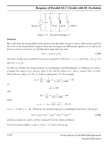
10u t A 32 : 10 H 1 640 F
e
0

Figure 1.11. Circuit for Example 1.3

Solution:
We could write the integrodifferential equation that describes the given circuit, differentiate, and find
the roots of the characteristic equation from the homogeneous differential equation as we did in the
previous section. However, we will skip these steps and start with
t
vt = v + v (1.49)
t
n
f
and when steady-state conditions have been reached we will have v = v = Ldi dt = 0 , v = 0

e

L
f
and vt = v .
t
n
To find out whether the natural response is overdamped, critically damped, or oscillatory, we need to
s
s
compute the values of D P and Z 0 using (1.43) and the values of and using (1.44) or (1.45).
2
1
Then will use (1.46), or (1.47), or (1.48) as appropriate. For this example,
G
1
1
D = ------- = ----------- = ------------------------------------- = 10
P
2C 2RC 2 u 32 u 1640
e
or
2
D = 100
P
and
1
1
2
Z = ------- = ---------------------------- = 64
0
LC 10 u 1 640
e
Then
2
2
s s 1 2 = – D P r D – Z = – 10 r 6
0
P
or s = – 4 and s = – 16 . Therefore, the natural response is overdamped and from (1.46) we get
2
1
s t s t
vt = v t = k e 1 + k e 2 = k e – 4t + k e – 16t (1.50)
2
2
1
1
n
and the constants and will be evaluated from the initial conditions.
k
k
2
1
From the initial condition v 0 = v0 = 5V and (1.50) we get
C
1-17 Circuit Analysis II with MATLAB Applications
Orchard Publications